
How to Map Wind Power Capacity by County
On this page
Problem statement
American wind power is concentrated: a few hundred rural counties in the plains, the Texas panhandle, the passes of California and the Columbia Gorge carry most of it. To map that, each turbine's rated capacity is summed by its county and joined to county boundaries. The US Wind Turbine Database already records the county of every turbine as a five-digit FIPS code, so the work is a groupby and a join, with three things to watch: the code must be read as text, a few thousand turbines have no capacity, and some codes belong to counties that no longer exist. This page maps version 9.1 by county.
Quick answer
Group the turbines by t_fips (read as text), sum t_cap (kilowatts) into megawatts, and merge onto the 2024 county boundaries by GEOID:
c = wt.groupby("t_fips").agg(turbines=("case_id", "size"), mw=("t_cap", lambda s: s.sum() / 1e3))
m = counties.merge(c, left_on="GEOID", right_index=True, how="left")
print(m.nlargest(6, "mw")[["NAME", "STUSPS", "turbines", "mw"]].round(0).to_string(index=False))
print(f"counties with turbines: {len(c)}; joined to a 2024 county: {m.mw.notna().sum()}")
NAME STUSPS turbines mw
Kern CA 3250.0 3254.0
Nolan TX 1349.0 2173.0
Willacy TX 680.0 1688.0
Gilliam OR 736.0 1612.0
Torrance NM 963.0 1595.0
Converse WY 645.0 1585.0
counties with turbines: 721; joined to a 2024 county: 717
Turbines stand in 721 counties, and 717 of the codes match a 2024 county. Kern County, California, has the most capacity, 3,254 MW from 3,250 turbines: Tehachapi Pass, with its old small turbines and new large ones side by side. The next five are in Texas, Oregon, New Mexico and Wyoming, each with 1,585 to 2,173 MW from far fewer turbines.
Summing, joining and the counties that changed
1. Turbines without a capacity
unknown = wt.t_cap.isna()
print(f"turbines without a capacity: {unknown.sum():,} ({unknown.mean():.1%}); summed capacity {wt.t_cap.sum() / 1e6:.1f} GW")
print(wt[unknown].groupby("t_state").size().nlargest(4).to_string())
turbines without a capacity: 5,056 (6.5%); summed capacity 159.6 GW
t_state
CA 1604
NM 1004
TX 739
CO 422
5,056 turbines, 6.5% of the file, have no capacity, so the county totals are a floor. They are not spread evenly: California has 1,604 of them and New Mexico 1,004, so their counties are understated most. A county map of turbine counts, which needs no capacity, is the check.
2. Codes that do not join
gone = c[~c.index.isin(counties.GEOID)]
print(gone.join(wt.groupby("t_fips").t_county.first()).to_string())
turbines mw t_county
t_fips
02270 14 2.000 Kusilvak
09005 2 5.700 Litchfield County
09009 1 0.100 New Haven County
66010 1 0.275 Guam
Connecticut's eight counties were replaced by nine planning regions in the Census Bureau's 2022 boundaries, so codes 09005 and 09009 exist only in older files. Alaska's Wade Hampton Census Area became Kusilvak in 2015 and got a new code, 02158; the turbine file has the new name under the old code. 66010 is Guam, which the county file leaves out. Only 18 turbines and 8.1 MW are affected, so they can be mapped by hand or left out.
3. Concentration
s = c.mw.sort_values(ascending=False)
share = s.cumsum() / s.sum()
print(f"counties holding half of the capacity: {(share < 0.5).sum() + 1}; 90%: {(share < 0.9).sum() + 1}; of {len(s)}")
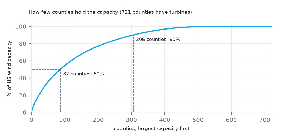
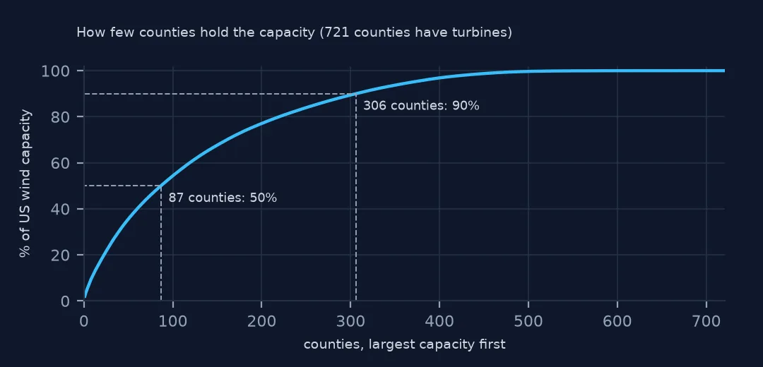
counties holding half of the capacity: 87; 90%: 306; of 721
Half of the country's wind capacity is in 87 counties, and 90% in 306 of the 721 counties that have any. Most US counties have no wind turbines at all.
Capacity per area, and a map
The data used on this page
The US Geological Survey's US Wind Turbine Database, version 9.1 of 28 September 2026 (Hoen and others, doi:10.5066/F7TX3DN0), public domain, saved on this site on 19 October 2026 because USGS replaces the file every quarter, and the Census Bureau's 2024 cartographic boundary counties (1:20 million).
from pathlib import Path
import zipfile

import geopandas as gpd
import pandas as pd
import requests

Path("data").mkdir(exist_ok=True)
# USGS US Wind Turbine Database v9.1 (28 September 2026) with its metadata and changelog, Census 2024 cartographic
# boundary counties and the EIA-860 2025 wind table. Saved 19 October 2026: USGS replaces the file every quarter.
# Live: https://energy.usgs.gov/uswtdb/assets/data/uswtdbCSV.zip
ARCHIVE = "usgs-uswtdb-v9-1-2026-10-19.zip"
if not Path(f"data/{ARCHIVE}").exists():
    Path(f"data/{ARCHIVE}").write_bytes(requests.get(f"https://data.spatialworkflow.io/{ARCHIVE}", timeout=600).content)
Z = zipfile.ZipFile(f"data/{ARCHIVE}")
wt = pd.read_csv(Z.open("uswtdb_V9_1_20260928.csv"), dtype={"t_fips": str})
Path("data/cb_2024_us_county_20m.zip").write_bytes(Z.read("cb_2024_us_county_20m.zip"))
counties = gpd.read_file("data/cb_2024_us_county_20m.zip")
print(f"US Wind Turbine Database v9.1: {len(wt):,} turbines; counties: {len(counties):,}")
US Wind Turbine Database v9.1: 77,839 turbines; counties: 3,222
Example 1: megawatts per 1,000 km²
m["km2"] = m.to_crs(5070).area / 1e6
m["mw_per_1000km2"] = m.mw / m.km2 * 1000
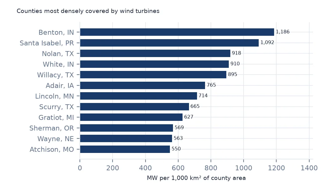
print(m.nlargest(5, "mw_per_1000km2")[["NAME", "STUSPS", "mw", "km2", "mw_per_1000km2"]].round(1).to_string(index=False))
NAME STUSPS mw km2 mw_per_1000km2
Benton IN 1249.2 1053.1 1186.3
Santa Isabel PR 101.2 92.7 1092.3
Nolan TX 2173.0 2366.4 918.3
White IN 1202.6 1321.7 910.0
Willacy TX 1687.7 1886.2 894.7
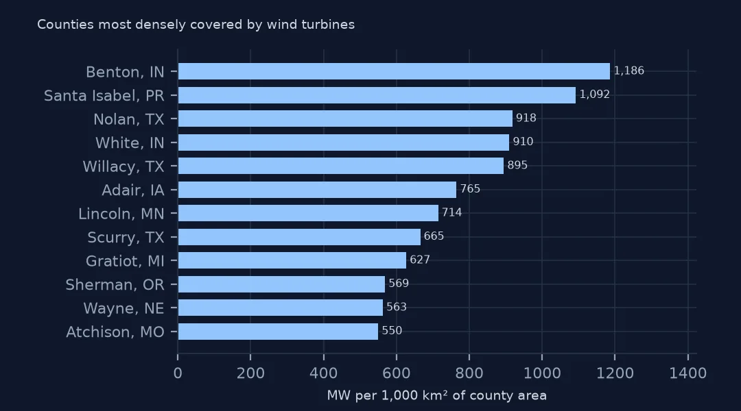
A large county can hold a lot of capacity and still be thinly covered. Divided by land area, Benton County, Indiana, ranks first, and Santa Isabel in Puerto Rico second, on the strength of a single 101 MW project in a small municipality.
Example 2: the choropleth
away = ["02", "15", "60", "66", "69", "72", "78"]
lower48 = m[~m.STATEFP.isin(away)].to_crs(5070)
ax = lower48.plot(column="mw", scheme="FisherJenks", k=6, cmap="YlGnBu", legend=True, figsize=(11, 6),
                  missing_kwds={"color": "#eeeeee"}, edgecolor="white", linewidth=0.1)
ax.set_axis_off()
print(f"lower 48 counties with turbines: {lower48.mw.notna().sum()}")
lower 48 counties with turbines: 695
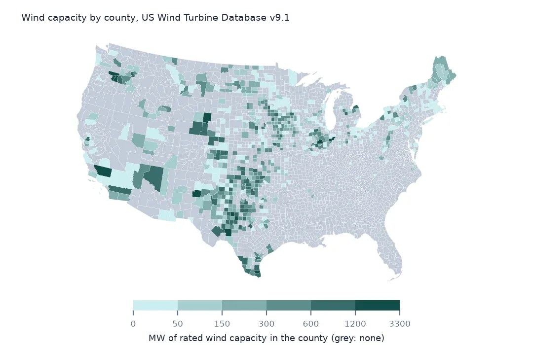
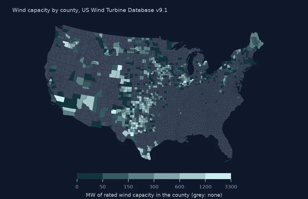
The map shows 695 counties of the lower 48 with turbines. Fisher-Jenks breaks suit a distribution this skewed, where most counties have a little and a few have more than a gigawatt. The dark band runs from west Texas up through Oklahoma, Kansas and Iowa, with separate dark patches in Wyoming, the Columbia Gorge and Kern County.
Internal links
- Reading the database — the columns and their units
- Project capacity summed per turbine — why
t_capis the column to sum - Turbines against EIA-860 — the capacity a county reports to EIA
- Choropleth classification — Fisher-Jenks and the other schemes