Weather Model Resolution Explained

On this page

Problem statement

A weather model's grid spacing sets the smallest feature it can represent, and it quietly shapes every number taken from it. A global model on a 27 km grid and a regional one on 3 km can both be "right" about the same storm and disagree by tens of knots at its centre, because each grid value is an average over its cell. Comparing models with each other, or with stations, means knowing what that average does to peaks, gradients and the places where land meets water.

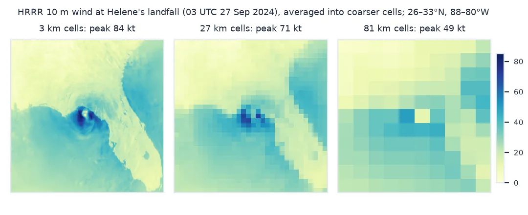
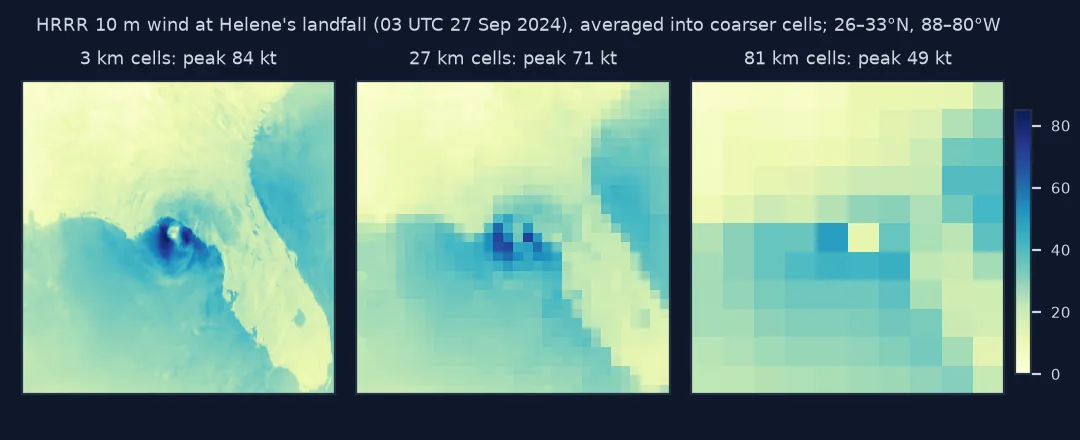
This page shows the effect directly by taking HRRR's 3 km analysis of Hurricane Helene at landfall, averaging it into coarser and coarser cells, and comparing the result with the 0.25° GFS and the National Hurricane Center's best track.

Quick answer

Average the wind components over blocks of grid cells and watch the peak fall:

def coarsen(a, k):
    ny, nx = (a.shape[0] // k) * k, (a.shape[1] // k) * k
    return a[:ny, :nx].reshape(ny // k, k, nx // k, k).mean(axis=(1, 3))

for k in (1, 3, 5, 9, 15, 27):
    peak = np.hypot(coarsen(U, k), coarsen(V, k)).max() * 1.94384
    print(f"{3 * k:>3} km cells: strongest 10 m wind {peak:5.1f} kt")
print(f"GFS 0.25° analysis, 3 hours earlier: {GFS_PEAK:.0f} kt; NHC best track at landfall: 120 kt")

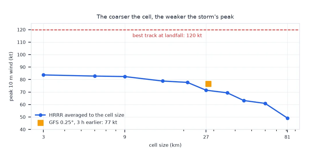
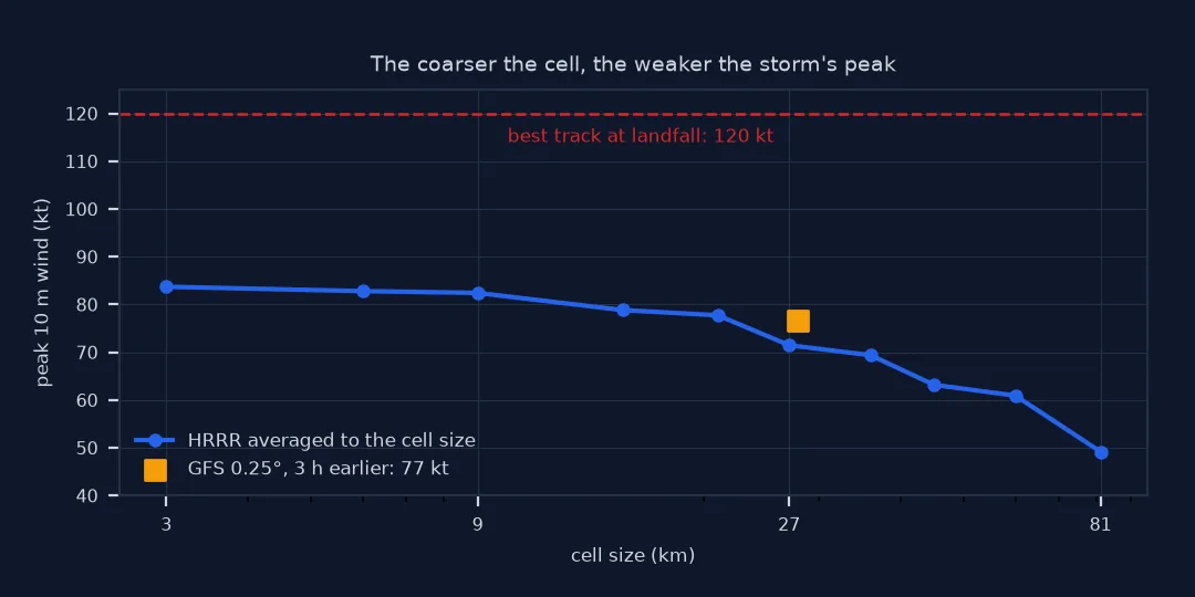
  3 km cells: strongest 10 m wind  83.7 kt
  9 km cells: strongest 10 m wind  82.4 kt
 15 km cells: strongest 10 m wind  78.8 kt
 27 km cells: strongest 10 m wind  71.5 kt
 45 km cells: strongest 10 m wind  63.2 kt
 81 km cells: strongest 10 m wind  49.2 kt
GFS 0.25° analysis, 3 hours earlier: 77 kt; NHC best track at landfall: 120 kt

Three panels of HRRR 10 m wind speed at Helene's landfall over the eastern Gulf and north Florida: at 3 kilometre cells a compact ring of winds up to 84 knots around a calm eye; averaged to 27 kilometre cells a blocky ring peaking at 71 knots; averaged to 81 kilometre cells a few large squares peaking at 49 knots with the eye merged into one cell. — The same storm at three cell sizes.

A grid value is an average, gradients sharpen, effective resolution

1. A grid value is an average

Each value in a model field represents its whole cell, not a point at its centre. Averaging the vector components over a larger cell is what a coarser model sees, and peaks smaller than the cell are spread out:

k = 9                                                                     # 9 × 3 km = 27 km, about the GFS cell
s3, s27 = np.hypot(U, V), np.hypot(coarsen(U, k), coarsen(V, k))
print(f"3 km cells above 64 kt: {(s3 * 1.94384 >= 64).sum()} ({(s3 * 1.94384 >= 64).sum() * 9:,} km²); "
      f"27 km cells above 64 kt: {(s27 * 1.94384 >= 64).sum()} ({(s27 * 1.94384 >= 64).sum() * 729:,} km²)")

3 km cells above 64 kt: 452 (4,068 km²); 27 km cells above 64 kt: 4 (2,916 km²)

2. Gradients sharpen with resolution

The change in wind across a short distance, at an eyewall or a coastline, is a gradient, and a coarse grid can only show gradients over its own spacing:

g3 = np.nanmax(np.abs(np.diff(s3, axis=1))) / 3
g27 = np.nanmax(np.abs(np.diff(s27, axis=1))) / 27
print(f"steepest east-west change in speed: {g3:.2f} m/s per km at 3 km, {g27:.2f} m/s per km at 27 km")

steepest east-west change in speed: 3.37 m/s per km at 3 km, 0.70 m/s per km at 27 km

Line chart of the peak 10 m wind against cell size on a logarithmic axis from 3 to 81 kilometres: 84 knots at 3, 82 at 9, 72 at 27 and 49 at 81, with the GFS at about 27 kilometres at 77 knots three hours earlier and the best track's 120 knots as a dashed line far above. — The coarser the cell, the weaker the peak.

3. Effective resolution is coarser than the grid

Models smooth features near their grid scale, so the smallest features they represent well are several grid lengths across, often quoted as four to seven grid spacings. Comparing the spread of values at each scale shows where the field loses its fine structure:

for k in (1, 3, 9, 27):
    s = np.hypot(coarsen(U, k), coarsen(V, k))
    print(f"{3 * k:>3} km: standard deviation of speed {s.std():.2f} m/s, 99th percentile {np.percentile(s, 99) * 1.94384:.0f} kt")

  3 km: standard deviation of speed 6.08 m/s, 99th percentile 57 kt
  9 km: standard deviation of speed 6.05 m/s, 99th percentile 57 kt
 27 km: standard deviation of speed 5.94 m/s, 99th percentile 53 kt
 81 km: standard deviation of speed 5.49 m/s, 99th percentile 44 kt

The same cell size from two models

The data used on this page

The HRRR 3 km analysis for 03 UTC on 27 September 2024 and the GFS 0.25° analysis for 00 UTC from AWS (HRRR, GFS), 10 m UGRD and VGRD, over 26–33°N, 88–80°W.

from pathlib import Path

import numpy as np
import requests
import xarray as xr

Path("data").mkdir(exist_ok=True)

def grib_wind(url, path):
    p = Path("data", path)
    if not p.exists():
        lines = requests.get(url + ".idx", timeout=60).text.splitlines()
        starts = [int(l.split(":")[1]) for l in lines]
        with open(p, "wb") as f:
            for i, l in enumerate(lines):
                if ":UGRD:10 m above ground:" in l or ":VGRD:10 m above ground:" in l:
                    f.write(requests.get(url, headers={"Range": f"bytes={starts[i]}-{starts[i + 1] - 1}"}, timeout=120).content)
    return xr.open_dataset(p, engine="cfgrib", decode_timedelta=False, backend_kwargs={
        "indexpath": "", "filter_by_keys": {"typeOfLevel": "heightAboveGround", "level": 10}}).load()

h = grib_wind("https://noaa-hrrr-bdp-pds.s3.amazonaws.com/hrrr.20240927/conus/hrrr.t03z.wrfsfcf00.grib2", "hrrr_helene_03z.grib2")
lat, lon = h.latitude.values, h.longitude.values - 360
ys, xs = np.where((lat > 26) & (lat < 33) & (lon > -88) & (lon < -80))
sub = h.isel(y=slice(ys.min(), ys.max() + 1), x=slice(xs.min(), xs.max() + 1))
U, V = sub.u10.values, sub.v10.values                                      # grid-relative: speeds and averages are unaffected
g = grib_wind("https://noaa-gfs-bdp-pds.s3.amazonaws.com/gfs.20240927/00/atmos/gfs.t00z.pgrb2.0p25.f000", "gfs_helene.grib2")
gs = g.sel(latitude=slice(33, 26), longitude=slice(272, 280))
GFS_PEAK = float(np.hypot(gs.u10, gs.v10).max()) * 1.94384
print(f"HRRR sub-grid {U.shape[0]} × {U.shape[1]} (3 km); GFS box {gs.u10.shape[0]} × {gs.u10.shape[1]} (0.25°)")

HRRR sub-grid 298 × 296 (3 km); GFS box 29 × 33 (0.25°)

Example 1: the same cell size, two models

At 27 km, the averaged HRRR and the GFS are both estimates of the storm at that scale, three hours apart:

print(f"HRRR averaged to 27 km: {np.hypot(coarsen(U, 9), coarsen(V, 9)).max() * 1.94384:.0f} kt; GFS on its 27 km grid: {GFS_PEAK:.0f} kt")

HRRR averaged to 27 km: 71 kt; GFS on its 27 km grid: 77 kt

At the same scale the two models are within 6 knots, with the GFS the stronger; three hours earlier, its storm was still over open water. Going from 3 km to 27 km cells costs HRRR 12 knots of peak wind; the 36 knots that still separate HRRR's own peak from the best track are the difference between any grid value and the strongest one-minute wind anywhere in the storm.

Grid spacing is not resolution

One storm, three cell sizes.

Grid spacing is the distance between the points where a model computes its values; resolution is the size of the smallest thing it represents faithfully, which is larger. A 27 km global model describes a hurricane's broad circulation well and its eyewall, a ring of maximum wind a few tens of kilometres wide, poorly: the strongest winds are averaged with weaker ones on either side. A 3 km model resolves the eyewall, and its peak values come much closer to observed extremes, though even it averages over 9 km² and over the model's time step.

This is why the same storm gives different "maximum winds" in different datasets, and why none matches a best-track intensity, which is the strongest one-minute wind anywhere in the storm. Comparisons are fair only between values at the same scale. Coarsening the fine model to the coarse grid, as here, is the simplest way to put them on equal terms; comparing a station with a grid cell always includes a difference of scale as well as of model error.

Averaging vectors, timing and nesting

Resolution traps.

Averaging vectors: average u and v, not speeds, when coarsening; averaging speeds keeps more of the peak but is not what a coarse model represents.
Grid-relative winds: rotation does not change speed, so speeds and coarse averages can use HRRR's grid-relative components as stored.
Time: models also average in time, over their time step; station gusts are a few seconds.
Different times: the GFS and HRRR analyses here are three hours apart, during which Helene moved inland.
Nested comparisons: block averaging assumes equal cell areas; HRRR's projection varies a few per cent across the domain.

Internal links

How to read HRRR wind data in Python — the 3 km model
How to check model winds against station observations — scale differences in verification

FAQ

What does weather model resolution mean?

Usually the grid spacing, the distance between grid points; the smallest features the model represents well are several times larger.

Why do global models underestimate hurricane winds?

Their grid cells, about 27 km for the GFS, average the narrow eyewall with weaker winds around it.

What is the resolution of HRRR and GFS?

HRRR runs at 3 km over the contiguous United States; the GFS is published on a 0.25° grid, about 27 km.

How do I compare models with different resolutions?

Average the finer model to the coarser grid, by block-averaging the wind components, and compare at the same scale.