How to Download GFS Wind Data From AWS in Python

On this page

Problem statement

NOAA's Global Forecast System (GFS) is the most widely used open weather model, and every run since 2021 is on Amazon S3, free and without an account. Each file is large: one forecast hour of the 0.25° GFS is about half a gigabyte, of which the 10-metre wind is a few megabytes. The files come with an index (.idx) listing the byte offset of every field, so a program can request only the fields it needs with HTTP range requests and never download the rest.

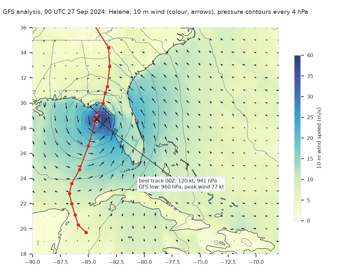
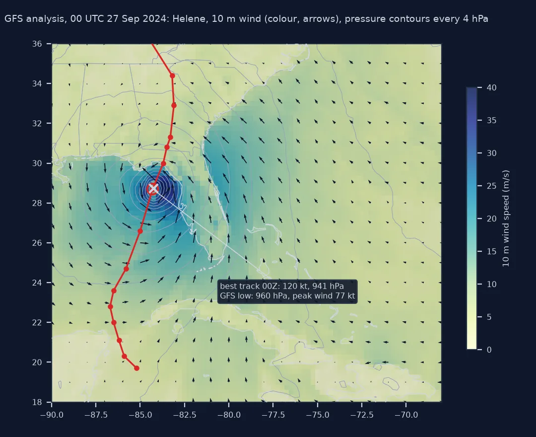
This page fetches the 10 m wind and sea-level pressure from the GFS analysis of 00 UTC on 27 September 2024, three hours before Hurricane Helene made landfall in Florida's Big Bend, opens them with cfgrib, and checks them against the National Hurricane Center's best track.

Quick answer

Read the index, request the byte ranges of the fields you want, and save them as one GRIB file:

def grib_subset(url, wanted, path):
    """Download only the GRIB messages whose index line contains one of `wanted` (e.g. 'UGRD:10 m above ground')."""
    lines = requests.get(url + ".idx", timeout=60).text.splitlines()
    starts = [int(line.split(":")[1]) for line in lines]
    with open(path, "wb") as f:
        for i, line in enumerate(lines):
            if any(f":{w}:" in line for w in wanted):
                end = starts[i + 1] - 1 if i + 1 < len(lines) else ""
                f.write(requests.get(url, headers={"Range": f"bytes={starts[i]}-{end}"}, timeout=120).content)
    return Path(path).stat().st_size

size = grib_subset(GFS, ["UGRD:10 m above ground", "VGRD:10 m above ground", "PRMSL:mean sea level"], "data/gfs_helene.grib2")
full = int(requests.head(GFS, timeout=60).headers["Content-Length"])
print(f"downloaded {size / 1e6:.1f} MB of a {full / 1e6:.0f} MB file ({size / full:.1%})")

downloaded 2.9 MB of a 506 MB file (0.6%)

Map of the Gulf of Mexico and the southeastern United States from 18 to 36 degrees north at 00 UTC on 27 September 2024: GFS 10 m wind speed shaded from 0 to 40 metres per second with arrows every fourth grid point and sea-level pressure contours every 4 hPa, showing a tight cyclone west of Florida with the strongest winds east of its centre; Helene's best track runs north from the Yucatán Channel to Georgia, and the GFS low, marked with a cross, sits on the best-track position; a label compares the best track's 120 knots and 941 hPa with the GFS low of 960 hPa and peak wind of 77 knots. — The GFS analysis puts Helene in the right place but cannot reproduce its strength.

Read the index, open the subset, crop and check against the track

1. Read the index

Find the two 10 m wind lines among the analysis file's messages; the quick answer took their byte ranges and the sea-level pressure's in the same way:

lines = requests.get(GFS + ".idx", timeout=60).text.splitlines()
print(f"{len(lines)} messages in the file")
print("\n".join(l for l in lines if ":10 m above ground:" in l and ("GRD" in l)))

696 messages in the file
585:417738655:d=2024092700:UGRD:10 m above ground:anl:
586:418709245:d=2024092700:VGRD:10 m above ground:anl:

Only the bytes you need.

2. Open the subset with cfgrib

The 10 m wind is on a heightAboveGround level and the pressure is a mean-sea-level field, so they open as two groups:

kw = {"indexpath": ""}                                                   # do not write .idx files next to the data
wind = xr.open_dataset("data/gfs_helene.grib2", engine="cfgrib", decode_timedelta=False,
                       backend_kwargs={**kw, "filter_by_keys": {"typeOfLevel": "heightAboveGround", "level": 10}}).load()
mslp = xr.open_dataset("data/gfs_helene.grib2", engine="cfgrib", decode_timedelta=False,
                       backend_kwargs={**kw, "filter_by_keys": {"shortName": "prmsl"}}).load()
print(f"variables: {list(wind.data_vars)} and {list(mslp.data_vars)}; grid {wind.sizes['latitude']} × {wind.sizes['longitude']}")
print(f"longitude runs {float(wind.longitude.min())} to {float(wind.longitude.max())}; latitude runs {float(wind.latitude[0])} to {float(wind.latitude[-1])}")

variables: ['u10', 'v10'] and ['prmsl']; grid 721 × 1440
longitude runs 0.0 to 359.75; latitude runs 90.0 to -90.0

The grid runs 0 to 359.75° east and from 90° north down to 90° south, so the Gulf of Mexico box in the next step is 270–292° east, written north to south. Why GRIB files need filters at all, and the other cfgrib traps, are in how to read GRIB weather data.

3. Crop, and check against the best track

box = dict(latitude=slice(36, 18), longitude=slice(270, 292))           # north to south, 0–360 longitudes
w = wind.sel(**box); p = mslp.prmsl.sel(**box) / 100
speed = np.hypot(w.u10, w.v10)
iy, ix = np.unravel_index(np.argmin(p.values), p.shape)
centre = (float(p.latitude[iy]), float(p.longitude[ix]) - 360)
bt = BEST.loc["2024-09-27 00:00"]
print(f"GFS low: {centre[0]:.2f}°N {abs(centre[1]):.2f}°W, {float(p.min()):.1f} hPa")
print(f"best track: {bt.lat:.1f}°N {abs(bt.lon):.1f}°W, {bt.pres:.0f} hPa, {bt.vmax:.0f} kt")
print(f"GFS strongest 10 m wind: {float(speed.max()):.1f} m/s = {float(speed.max()) * 1.94384:.0f} kt")

GFS low: 28.75°N 84.25°W, 960.4 hPa
best track: 28.7°N 84.3°W, 941 hPa, 120 kt
GFS strongest 10 m wind: 39.4 m/s = 77 kt

Right place, too weak.

The analysis puts the storm in the right place, to within a grid cell, but at 0.25°, about 27 km, it cannot resolve a hurricane's eyewall: its lowest pressure and strongest wind fall well short of the best track. For a storm's core, use a convection-allowing model such as HRRR, or the best track itself.

Other levels and a forecast with the same function

The data used on this page

The NOAA GFS on AWS open data bucket (noaa-gfs-bdp-pds), 0.25° analysis (f000) of the 00 UTC run on 27 September 2024, and the National Hurricane Center's best track for Hurricane Helene (AL09) in ATCF format: position, maximum sustained wind (knots) and central pressure every six hours.

import gzip
from pathlib import Path

import numpy as np
import pandas as pd
import requests
import xarray as xr

Path("data").mkdir(exist_ok=True)
GFS = "https://noaa-gfs-bdp-pds.s3.amazonaws.com/gfs.20240927/00/atmos/gfs.t00z.pgrb2.0p25.f000"
F = Path("data/bal092024.dat.gz")
if not F.exists():
    F.write_bytes(requests.get("https://ftp.nhc.noaa.gov/atcf/archive/2024/bal092024.dat.gz", timeout=60).content)
cols = ["basin", "num", "time", "tech_num", "tech", "tau", "lat", "lon", "vmax", "pres", "type"]
bt = pd.read_csv(gzip.open(F, "rt"), header=None, usecols=range(11), names=cols, skipinitialspace=True, dtype=str)
bt["time"] = pd.to_datetime(bt.time, format="%Y%m%d%H")
bt["lat"] = bt.lat.str[:-1].astype(float) / 10 * np.where(bt.lat.str[-1] == "N", 1, -1)
bt["lon"] = bt.lon.str[:-1].astype(float) / 10 * np.where(bt.lon.str[-1] == "E", 1, -1)
BEST = bt.drop_duplicates("time").set_index("time")[["lat", "lon", "vmax", "pres", "type"]].astype({"vmax": int, "pres": int})
print(f"Helene best track: {len(BEST)} positions, {BEST.index.min():%d %b %H}Z to {BEST.index.max():%d %b %H}Z; peak {BEST.vmax.max()} kt")

Helene best track: 25 positions, 23 Sep 12Z to 28 Sep 18Z; peak 120 kt

Example 1: other levels with the same function

The jet stream at 250 hPa is two more index lines:

grib_subset(GFS, ["UGRD:250 mb", "VGRD:250 mb"], "data/gfs_250mb.grib2")
jet = xr.open_dataset("data/gfs_250mb.grib2", engine="cfgrib", decode_timedelta=False,
                      backend_kwargs={"indexpath": "", "filter_by_keys": {"typeOfLevel": "isobaricInhPa"}}).load()
s250 = np.hypot(jet.u, jet.v).sel(latitude=slice(60, 20), longitude=slice(230, 300))
print(f"250 hPa over North America: strongest {float(s250.max()):.0f} m/s; levels in file: {jet.isobaricInhPa.values}")

250 hPa over North America: strongest 77 m/s; levels in file: 250.0

Example 2: a forecast instead of the analysis

Forecast files differ only in the last part of the name, f000 to f384; f024 from this run is the forecast for 00 UTC on 28 September:

f24 = GFS.replace("f000", "f024")
print([l for l in requests.get(f24 + ".idx", timeout=60).text.splitlines() if "UGRD:10 m above ground" in l])

['588:433411178:d=2024092700:UGRD:10 m above ground:24 hour fcst:']

Right place, too weak: what a 0.25° analysis can see

The analysis and the best track disagree because they measure different things. A GFS grid value is an average over a cell about 27 km across, and a hurricane's strongest winds sit in an eyewall ring a few tens of kilometres wide, so the grid smears the peak across its neighbours: Helene's analysed low was 960.4 hPa against the best track's 941, and its strongest 10 m wind 77 kt against 120. The best track's wind is a one-minute sustained maximum at a point, the analysis's a grid-cell value. Position survives the smoothing far better than intensity, which is why the low sat within a grid cell of the best-track centre.

The GFS analysis (f000) is the model's best estimate of the atmosphere at the run time, blending observations into a short forecast. It is a gridded estimate, smooth at the scale of its grid. Comparing it with independent data, such as the best track here or station observations, is part of using it, not an extra.

Availability, variable names and units

GFS download traps.

Availability: the AWS bucket holds GFS from 2021 onward; older runs are at NCEI.
The last message: its range has no end; request bytes=start- for it.
Variable names: cfgrib renames fields (UGRD at 10 m becomes u10, PRMSL becomes prmsl); look at data_vars after opening.
Units: winds are m/s; multiply by 1.94384 for knots, the unit of the best track.

Internal links

How to read GRIB weather data in Python — GRIB and cfgrib in general
Why won't my GRIB file open with cfgrib? — errors when opening

FAQ

How do I download only some variables from a GFS file?

Read the .idx file next to it, find the byte offsets of the fields you want, and request those ranges with an HTTP Range header.

Where is GFS data on AWS?

In the public bucket noaa-gfs-bdp-pds, under gfs.YYYYMMDD/HH/atmos/, readable over HTTPS without an account.

Why does GFS underestimate hurricane winds?

Its 0.25° grid, about 27 km, is too coarse to resolve the eyewall, so peak winds and the lowest pressure are smoothed out.

What does f000 mean in a GFS file name?

The forecast hour: f000 is the analysis at the run time, f024 the forecast 24 hours later.