
How to Map the Jet Stream in Python
On this page
Problem statement
The jet stream is the band of fastest wind near the top of the troposphere, about 10 kilometres up, and its position steers weather systems below it. Maps of it are drawn on a pressure level, usually 250 hPa, from the wind components and the geopotential height there: the height contours show the troughs and ridges, and isotachs of wind speed show the jet and the faster "streaks" within it. Getting there from a model file means picking the right level, keeping the heights in metres, and deciding what speed counts as "jet".
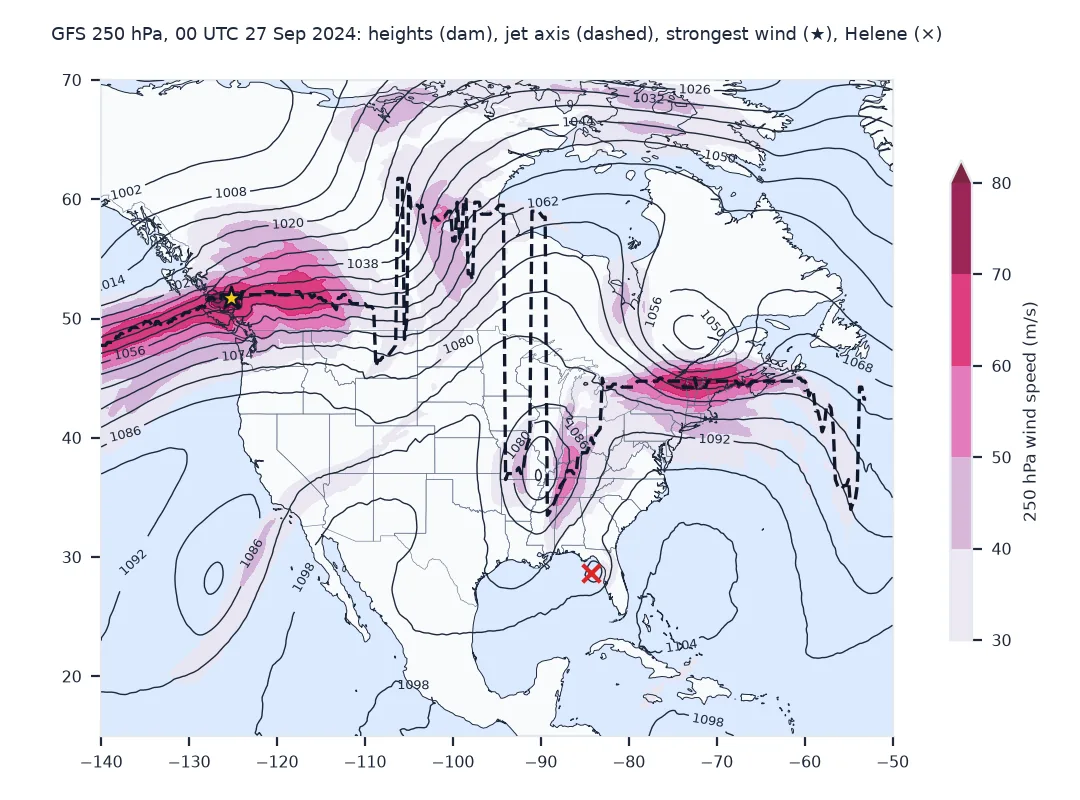
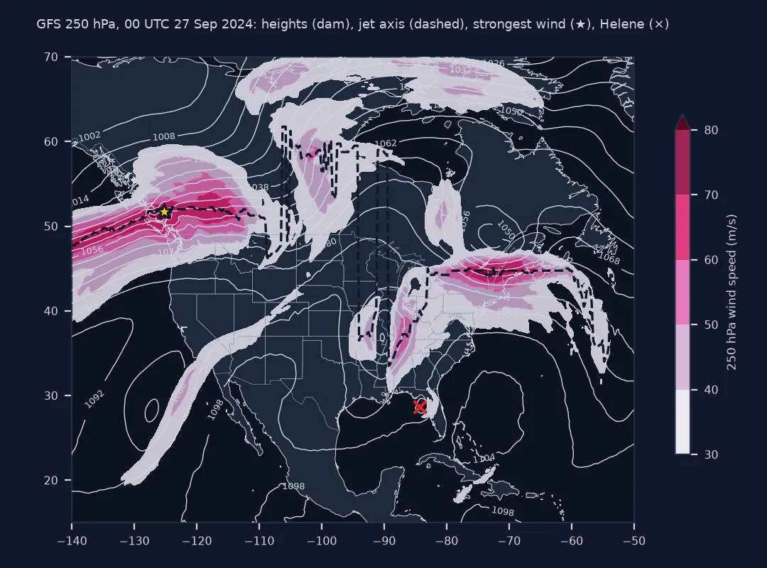
This page maps the GFS analysis at 250 hPa over North America for 00 UTC on 27 September 2024, finds the strongest jet streak, traces the jet axis, and locates the closed low over the eastern United States that sat north of Hurricane Helene's path.
Quick answer
Download UGRD, VGRD and HGT at 250 mb by byte range, compute speed, and contour height over the speed:
w = J.sel(latitude=slice(70, 15), longitude=slice(220, 310))
speed = np.hypot(w.u, w.v)
iy, ix = np.unravel_index(int(np.argmax(speed.values)), speed.shape)
print(f"strongest 250 hPa wind: {float(speed.max()):.1f} m/s ({float(speed.max()) * 1.94384:.0f} kt) at "
      f"{float(w.latitude[iy]):.2f}°N {360 - float(w.longitude[ix]):.2f}°W")
cell_km2 = (111.195 * 0.25) ** 2 * np.cos(np.radians(w.latitude))
print(f"area with winds above 50 m/s: {float(cell_km2.where(speed > 50).sum()):,.0f} km²")
print(f"250 hPa heights: {float(w.gh.min()):,.0f} to {float(w.gh.max()):,.0f} m")
strongest 250 hPa wind: 76.6 m/s (149 kt) at 51.75°N 125.25°W
area with winds above 50 m/s: 1,560,701 km²
250 hPa heights: 9,992 to 11,056 m
One pressure level, the jet axis, the closed low
1. Fetch one pressure level
GFS files hold winds and heights on many pressure levels; the index lines carry the level, so :250 mb: picks exactly the jet level:
lines = requests.get(GFS + ".idx", timeout=60).text.splitlines()
print("\n".join(l for l in lines if ":250 mb:" in l and any(v in l for v in ("UGRD", "VGRD", "HGT"))))
print(f"levels with UGRD in the file: {sum(':UGRD:' in l and ' mb:' in l for l in lines)}")
269:203841899:d=2024092700:HGT:250 mb:anl:
276:209891015:d=2024092700:UGRD:250 mb:anl:
277:210489816:d=2024092700:VGRD:250 mb:anl:
levels with UGRD in the file: 41
2. Trace the jet axis
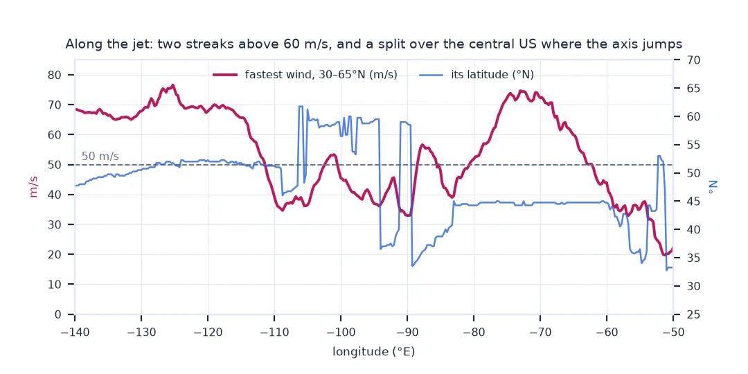
The jet axis is the line of maximum wind. A simple version takes, for each longitude, the latitude of the fastest wind between 30° and 65°N, where it exceeds 30 m/s:
band = speed.sel(latitude=slice(65, 30))
lat_max = band.idxmax("latitude"); v_max = band.max("latitude")
axis = pd.DataFrame({"lon": band.longitude.values - 360, "lat": lat_max.values, "speed": v_max.values})
axis = axis[axis.speed > 30]
print(f"jet axis found at {len(axis)} of {band.sizes['longitude']} longitudes; latitude range {axis.lat.min()}–{axis.lat.max()}°N")
print(axis.iloc[::40].round(1).to_string(index=False))
jet axis found at 349 of 361 longitudes; latitude range 33.5–61.75°N
lon lat speed
-140.0 47.8 68.500000
-130.0 50.5 67.800003
-120.0 52.2 67.800003
-110.0 51.2 39.400002
-100.0 56.5 45.599998
-90.0 58.8 33.000000
-80.0 44.2 51.900002
-70.0 44.8 72.300003
-60.0 44.8 43.900002
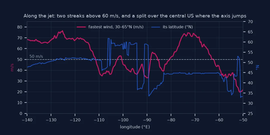
Where the flow is weak or split, as over the central United States here, the fastest wind in each column jumps between latitudes, and the line zigzags. A higher threshold, or following the axis from one longitude to the next, gives a cleaner line.
3. Find the closed low
A closed low is a minimum of height enclosed by contours. Over the eastern United States the lowest 250 hPa height at this time was:
east = w.gh.sel(latitude=slice(45, 30), longitude=slice(265, 285))
jy, jx = np.unravel_index(int(np.argmin(east.values)), east.shape)
print(f"lowest height {float(east.min()):,.0f} m at {float(east.latitude[jy]):.2f}°N {360 - float(east.longitude[jx]):.2f}°W; "
      f"Helene's best-track centre at 00 UTC: 28.7°N 84.3°W")
lowest height 10,679 m at 36.75°N 90.25°W; Helene's best-track centre at 00 UTC: 28.7°N 84.3°W
Jet speeds in knots for aviation
The data used on this page
The GFS 0.25° analysis for 00 UTC on 27 September 2024 from the NOAA GFS bucket on AWS: UGRD, VGRD and HGT at 250 mb, opened with cfgrib.
from pathlib import Path

import numpy as np
import pandas as pd
import requests
import xarray as xr

Path("data").mkdir(exist_ok=True)
GFS = "https://noaa-gfs-bdp-pds.s3.amazonaws.com/gfs.20240927/00/atmos/gfs.t00z.pgrb2.0p25.f000"
F = Path("data/gfs_250mb.grib2")
if not F.exists():
    lines = requests.get(GFS + ".idx", timeout=60).text.splitlines()
    starts = [int(l.split(":")[1]) for l in lines]
    with open(F, "wb") as f:
        for i, l in enumerate(lines):
            if any(f":{v}:250 mb:" in l for v in ("UGRD", "VGRD", "HGT")):
                f.write(requests.get(GFS, headers={"Range": f"bytes={starts[i]}-{starts[i + 1] - 1}"}, timeout=120).content)
J = xr.open_dataset(F, engine="cfgrib", decode_timedelta=False, backend_kwargs={
    "indexpath": "", "filter_by_keys": {"typeOfLevel": "isobaricInhPa"}}).load()
print(f"variables {list(J.data_vars)} at {float(J.isobaricInhPa):.0f} hPa; gh units: {J.gh.attrs.get('units')}")
variables ['gh', 'u', 'v'] at 250 hPa; gh units: gpm
Example 1: speed in knots for aviation
Aviation charts give jet speeds in knots and mark cores above 80 kt:
kt = speed * 1.94384
print(f"grid points above 80 kt: {int((kt > 80).sum()):,}; above 120 kt: {int((kt > 120).sum()):,}")
grid points above 80 kt: 6,479; above 120 kt: 1,094
Where the jet stream sits, and why
The jet stream sits where the temperature contrast between polar and tropical air is concentrated: the steeper the contrast below, the faster the wind above. On a constant-pressure map, the wind blows nearly parallel to the height contours, faster where they are packed together, which is why the two fields are drawn together. Speeds above about 50 m/s mark the jet; streaks within it, regions of locally faster wind, are where the strongest weather systems tend to develop.
Closed lows at this level are pools of cold air cut off from the main flow. They move slowly and influence the steering of storms beneath and around them. Here the lowest heights over the east lay near where Missouri, Kentucky and Tennessee meet, about 1,000 km north-west of Helene's centre.
Geopotential units and level choice
- Height units: GFS
HGTis geopotential metres; maps often label it in decametres (divide by 10). - Level choice: 250 hPa suits mid-latitudes in most seasons; 200 hPa is closer to the jet in the tropics and in summer, 300 hPa in winter.
- Thresholds: 50 m/s, about 100 kt, is a common jet threshold; aviation uses 80 kt for jet cores.
- Longitude: GFS longitudes run 0–360; North America is about 190–310.
- Projection: for hemispheric maps, use a polar stereographic or Lambert projection and rotate the winds.
Internal links
- How to download GFS wind data from AWS — byte-range downloads
- How to draw wind streamlines in Python — another way to draw the flow
FAQ
How do I plot the jet stream in Python?
Download u, v and geopotential height at 250 hPa, compute speed with np.hypot(u, v), shade speeds above about 50 m/s and contour the heights.
What pressure level is the jet stream?
Usually drawn at 250 hPa, about 10 to 11 km up; 200 or 300 hPa can be better depending on season and latitude.
How fast is the jet stream?
Typically 50 to 80 m/s in its core; here the strongest wind over North America was 76.6 m/s, about 149 knots.
What is a jet streak?
A region of locally faster wind within the jet stream, often where storms develop.