How to Calculate Vorticity and Divergence From Wind in Python

Problem statement

Vorticity measures how much the wind rotates; divergence measures how much it spreads out or, when negative, converges. Both are derivatives of the wind field, and both pick out structure that wind speed hides: the spin at the centre of a low, a line of convergence along a front, the outflow at the top of a storm. Computing them on a latitude-longitude grid needs the grid spacing in metres, which shrinks towards the poles, and a sign convention, so that "positive" means cyclonic in the Northern Hemisphere.

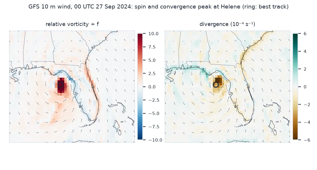
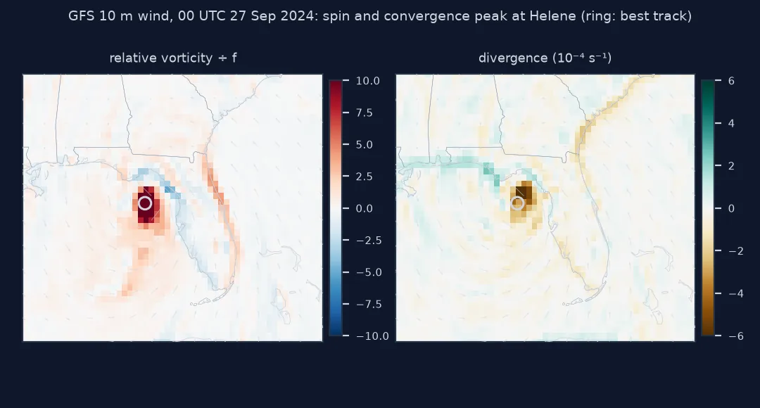
This page computes relative vorticity and divergence of the GFS 10-metre wind at 00 UTC on 27 September 2024 with MetPy, finds Hurricane Helene's centre from them, and checks MetPy against a few lines of NumPy.

Quick answer

Let MetPy take the grid spacing from the coordinates:

u, v = W.u10.metpy.quantify(), W.v10.metpy.quantify()
vort = mpcalc.vorticity(u, v).metpy.dequantify()             # s⁻¹, positive = anticlockwise (cyclonic in the north)
div = mpcalc.divergence(u, v).metpy.dequantify()             # s⁻¹, negative = converging
iv = np.unravel_index(np.nanargmax(vort.values), vort.shape)
idv = np.unravel_index(np.nanargmin(div.values), div.shape)
print(f"strongest cyclonic vorticity {vort.values[iv]:.2e} s⁻¹ at {LAT[iv[0]]}°N {abs(LON[iv[1]])}°W")
print(f"strongest convergence {div.values[idv]:.2e} s⁻¹ at {LAT[idv[0]]}°N {abs(LON[idv[1]])}°W")
print(f"best track at 00 UTC: {BT.lat}°N {abs(BT.lon)}°W")

strongest cyclonic vorticity 1.51e-03 s⁻¹ at 28.75°N 84.25°W
strongest convergence -8.97e-04 s⁻¹ at 29.25°N 84.25°W
best track at 00 UTC: 28.7°N 84.3°W

What the numbers mean, a hand check, no flat-degree grids

1. Know what the numbers mean

Vorticity is in s⁻¹. A useful yardstick is the Coriolis parameter f, the vorticity the earth's rotation gives the air at that latitude; weather systems have relative vorticity of the order of f, a mature hurricane many times it:

f = 2 * 7.2921e-5 * np.sin(np.radians(LAT[iv[0]]))
print(f"f at {LAT[iv[0]]}°N: {f:.2e} s⁻¹; Helene's peak relative vorticity is {vort.values[iv] / f:.1f} f")
print(f"grid points with vorticity above f: {(vort.values > f).sum()}; above 10 f: {(vort.values > 10 * f).sum()}")

f at 28.75°N: 7.01e-05 s⁻¹; Helene's peak relative vorticity is 21.5 f
grid points with vorticity above f: 476; above 10 f: 13

2. Check the calculation by hand

On a sphere, ζ = (1 / R cos φ) · (∂v/∂λ − ∂(u cos φ)/∂φ). NumPy's gradient with the coordinates in radians does the derivatives:

R = 6371229.0
lat, lon = np.radians(LAT), np.radians(LON)
dv_dlon = np.gradient(W.v10.values, lon, axis=1)
ducos_dlat = np.gradient(W.u10.values * np.cos(lat)[:, None], lat, axis=0)
zeta = (dv_dlon - ducos_dlat) / (R * np.cos(lat)[:, None])
inner = (slice(2, -2), slice(2, -2))                                    # the edges use one-sided differences
print(f"NumPy peak {np.nanmax(zeta[inner]):.4e}, MetPy peak {np.nanmax(vort.values[inner]):.4e}; "
      f"largest difference {np.nanmax(np.abs(zeta[inner] - vort.values[inner])):.1e} s⁻¹")

NumPy peak 1.5101e-03, MetPy peak 1.5111e-03; largest difference 3.1e-06 s⁻¹

3. Do not treat degrees as a flat grid

Using a constant 111 km per degree in both directions ignores the shrinking of longitude: at 28.75°N the east-west spacing is overestimated by 14%, so the ∂v/∂x term comes out 12% too small, while the ∂u/∂y term is unaffected:

dx_flat = 111_195.0 * np.gradient(LON)                                   # metres per grid step, wrongly constant
dy = 111_195.0 * np.gradient(LAT)
zeta_flat = np.gradient(W.v10.values, axis=1) / dx_flat[None, :] - np.gradient(W.u10.values, axis=0) / dy[:, None]
print(f"peak with flat degrees {np.nanmax(zeta_flat[inner]):.3e} against {np.nanmax(vort.values[inner]):.3e} "
      f"({np.nanmax(zeta_flat[inner]) / np.nanmax(vort.values[inner]) - 1:+.0%})")

peak with flat degrees 1.375e-03 against 1.511e-03 (-9%)

The peak is 9% too low here, and the error grows towards the poles, so it distorts every comparison between latitudes.

Smoothing first, and circulation around the storm

The data used on this page

The GFS 0.25° analysis for 00 UTC on 27 September 2024 from the NOAA GFS bucket on AWS, 10 m UGRD and VGRD, cut to 14–40°N and 98–60°W, and the NHC best track for Hurricane Helene.

import gzip
from pathlib import Path

import metpy.calc as mpcalc
import numpy as np
import pandas as pd
import requests
import xarray as xr

Path("data").mkdir(exist_ok=True)
GFS = "https://noaa-gfs-bdp-pds.s3.amazonaws.com/gfs.20240927/00/atmos/gfs.t00z.pgrb2.0p25.f000"
G = Path("data/gfs_helene.grib2")
if not G.exists():
    lines = requests.get(GFS + ".idx", timeout=60).text.splitlines()
    starts = [int(l.split(":")[1]) for l in lines]
    with open(G, "wb") as f:
        for i, l in enumerate(lines):
            if ":UGRD:10 m above ground:" in l or ":VGRD:10 m above ground:" in l:
                f.write(requests.get(GFS, headers={"Range": f"bytes={starts[i]}-{starts[i + 1] - 1}"}, timeout=120).content)
ds = xr.open_dataset(G, engine="cfgrib", decode_timedelta=False, backend_kwargs={
    "indexpath": "", "filter_by_keys": {"typeOfLevel": "heightAboveGround", "level": 10}}).load()
W = ds.sel(latitude=slice(40, 14), longitude=slice(262, 300))
LAT, LON = W.latitude.values, W.longitude.values - 360
B = Path("data/bal092024.dat.gz")
if not B.exists():
    B.write_bytes(requests.get("https://ftp.nhc.noaa.gov/atcf/archive/2024/bal092024.dat.gz", timeout=60).content)
bt = pd.read_csv(gzip.open(B, "rt"), header=None, usecols=[2, 6, 7], names=["time", "lat", "lon"], skipinitialspace=True, dtype=str)
bt = bt[bt.time == "2024092700"].iloc[0]
BT = pd.Series({"lat": float(bt.lat[:-1]) / 10, "lon": -float(bt.lon[:-1]) / 10})
print(f"{W.sizes['latitude']} × {W.sizes['longitude']} grid; {LAT.max()}–{LAT.min()}°N")

105 × 153 grid; 40.0–14.0°N

Example 1: smoothing before differentiating

Derivatives amplify noise. A light smoothing, here a 9-point filter, keeps the large structures and lowers the extremes:

vort_s = mpcalc.smooth_n_point(vort, 9, 2)
print(f"peak before {np.nanmax(vort.values):.2e}, after two passes of a 9-point smoother {np.nanmax(vort_s.values):.2e} s⁻¹")

peak before 1.51e-03, after two passes of a 9-point smoother 1.07e-03 s⁻¹

Example 2: the circulation around the storm

Vorticity integrated over an area is the circulation around its edge; over a box 4° on a side centred on the storm:

box = (abs(LAT[:, None] - BT.lat) <= 2) & (abs(LON[None, :] - BT.lon) <= 2)
dy_m = 111_195.0 * 0.25
dx_m = dy_m * np.cos(np.radians(LAT))[:, None] * np.ones_like(box)
circ = np.nansum(vort.values[box] * (dx_m[box] * dy_m))
print(f"circulation {circ:.2e} m²/s; mean vorticity in the box {np.nanmean(vort.values[box]):.2e} s⁻¹")

circulation 1.84e+07 m²/s; mean vorticity in the box 1.06e-04 s⁻¹

Curl and divergence of the wind

Relative vorticity is the curl of the horizontal wind, ∂v/∂x − ∂u/∂y: positive where the wind turns anticlockwise, which is cyclonic in the Northern Hemisphere. Divergence is ∂u/∂x + ∂v/∂y: negative where air piles in, as it does into a low near the surface, where it must rise. A hurricane shows both near its centre: intense cyclonic vorticity and strong low-level convergence, the second slightly offset from the first here, half a degree to the north.

On a sphere the derivatives need the metric terms: the east-west distance between grid columns is R cos φ Δλ, and the u cos φ term accounts for the convergence of the meridians. MetPy handles this when it is given latitude and longitude coordinates with units. Values on a 0.25° grid are averages over 27 km; a finer model resolves stronger peaks, so vorticity magnitudes are only comparable between data at the same resolution.

Units, edges and hemispheres

• Units: MetPy needs u and v with units; .metpy.quantify() reads them from the GRIB attributes.
• Edges: the outermost row and column use one-sided differences; trim them before reporting extremes.
• Southern Hemisphere: cyclonic vorticity is negative there; absolute vorticity adds f.
• Projected grids: on HRRR's grid, use the grid spacing in metres and grid-relative winds together, or rotate first and use lat_lon_grid_deltas.
• Levels: vorticity at 850 or 500 hPa is the usual analysis level; near-surface values are noisier.

Internal links

• How to download GFS wind data from AWS — the wind field
• How to draw wind streamlines in Python — the rotation, drawn

FAQ

How do I calculate vorticity in Python?

Use metpy.calc.vorticity(u, v) on xarray data with latitude and longitude coordinates and units; it handles the spherical grid spacing.

What units does vorticity have?

Inverse seconds (s⁻¹); typical values are 10⁻⁵ to 10⁻⁴ s⁻¹, and hurricanes reach 10⁻³ s⁻¹ near their centres.

What does negative divergence mean?

Convergence: air flowing into the area, which near the surface forces it to rise.

Why does my vorticity look wrong on a latitude-longitude grid?

The grid spacing was treated as constant in metres; the east-west spacing shrinks with the cosine of latitude.