How to Build a Hedonic Price Model for Airbnb Listings in Python

On this page

Problem statement

Why does one listing cost $150 a night and another $400? A hedonic price model answers by splitting a price into the value of its characteristics: bedrooms, bathrooms, room type, location, reviews. It is the standard tool for housing prices, and with Inside Airbnb data it takes a few lines of statsmodels. Getting a model that means something takes more: log prices so effects are proportional, categorical variables coded properly, outliers handled with a stated rule, and location in the model so that a "bedroom effect" is not secretly a "downtown effect".

This page fits a hedonic model of nightly price for the Inside Airbnb listings of Washington, D.C. from the snapshot of 24 June 2026. It adds variables step by step, reads the coefficients as percentages, adds neighbourhood fixed effects, and checks how well the model predicts listings it has not seen.

Quick answer

Regress log price on characteristics with categorical room type:

import statsmodels.formula.api as smf
m1 = smf.ols("log_price ~ bedrooms + bathrooms + accommodates + C(room_type)", data=D).fit()
pct = lambda b: 100 * (np.exp(b) - 1)
print(f"n = {int(m1.nobs):,}; R² = {m1.rsquared:.3f}")
for v in ("bedrooms", "bathrooms", "accommodates"):
    print(f"{v:>13}: {pct(m1.params[v]):+.1f}% per unit (95% CI {pct(m1.conf_int().loc[v, 0]):+.1f} to {pct(m1.conf_int().loc[v, 1]):+.1f}%)")

n = 5,126; R² = 0.317
     bedrooms: +2.7% per unit (95% CI -0.3 to +5.8%)
    bathrooms: +14.1% per unit (95% CI +10.5 to +17.9%)
 accommodates: +8.7% per unit (95% CI +7.6 to +9.8%)

Size and room type explain 32% of the variation in log price. Each extra guest of capacity adds 8.7%, and each bathroom 14.1%. A bedroom adds only 2.7%, with an interval that includes zero, because capacity already captures most of what bedrooms do.

R² rises from 0.317 to 0.471 with neighbourhoods and to 0.678 with more terms.

Add location, reviews and host status, an out-of-sample check

1. Add location

Neighbourhood fixed effects absorb everything about each area. Compare the coefficients with and without them:

m2 = smf.ols("log_price ~ bedrooms + bathrooms + accommodates + C(room_type) + C(neighbourhood_cleansed)", data=D).fit()
print(f"R² without location {m1.rsquared:.3f}, with neighbourhood effects {m2.rsquared:.3f}")
print(f"bedroom effect: {pct(m1.params['bedrooms']):+.1f}% without location, {pct(m2.params['bedrooms']):+.1f}% with")
nb = m2.params.filter(like="neighbourhood_cleansed").sort_values()
print(f"neighbourhood effects range {pct(nb.min()):+.0f}% to {pct(nb.max()):+.0f}% relative to the reference area ({D.neighbourhood_cleansed.sort_values().iloc[0][:30]})")

R² without location 0.317, with neighbourhood effects 0.471
bedroom effect: +2.7% without location, +9.9% with
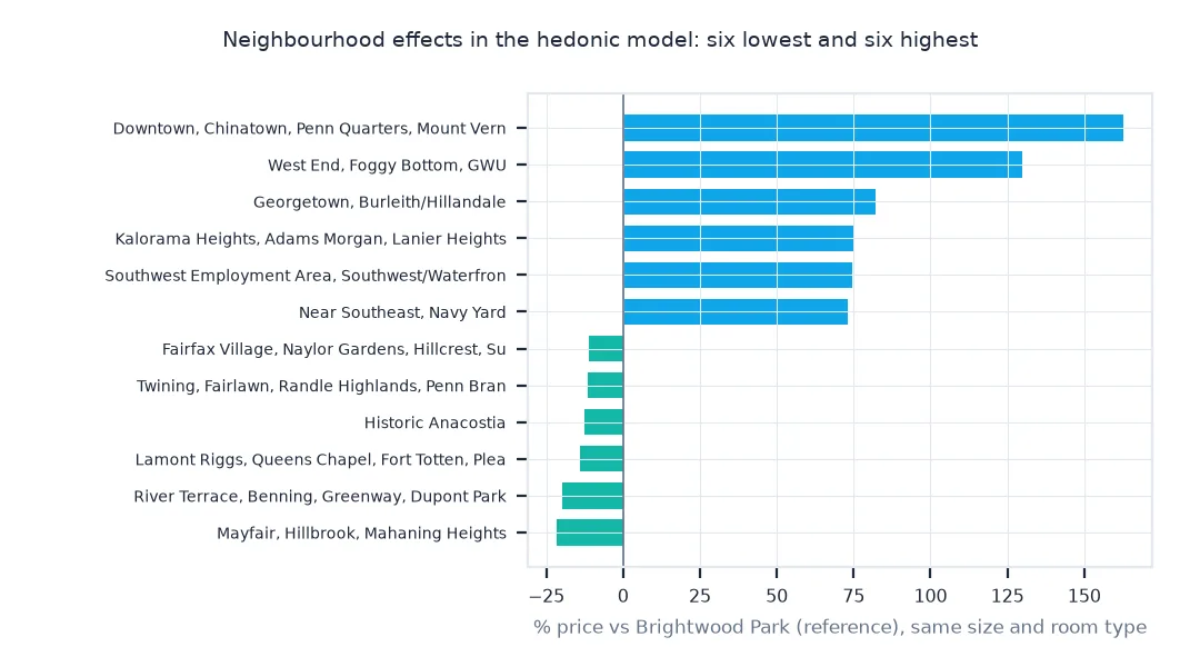
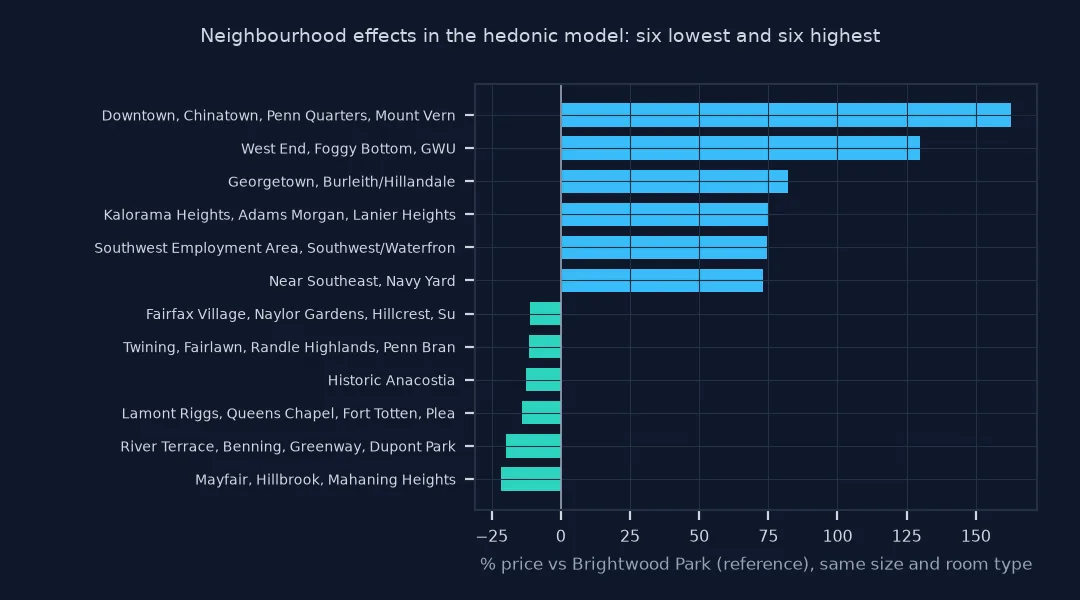
neighbourhood effects range -22% to +163% relative to the reference area (Brightwood Park, Crestwood, Pe)

Adding neighbourhoods lifts the R² from 0.317 to 0.471, and the bedroom effect more than triples, to 9.9%. That is consistent with larger homes sitting in cheaper outer neighbourhoods, which hides the value of a bedroom when location is left out. Relative to the reference area, Brightwood Park, Crestwood and Petworth, neighbourhoods range from 22% cheaper to 163% dearer.

The bedroom effect grows from +2.7% to +9.9% once location is controlled.

2. Reviews and host status

m3 = smf.ols("log_price ~ bedrooms + bathrooms + accommodates + C(room_type) + C(neighbourhood_cleansed) + review_scores_rating + C(host_is_superhost) + long_stay", data=D.dropna(subset=["review_scores_rating", "host_is_superhost"])).fit()
for v in ("review_scores_rating", "C(host_is_superhost)[T.t]", "long_stay"):
    print(f"{v:>26}: {pct(m3.params[v]):+.1f}% (p = {m3.pvalues[v]:.3f})")
print(f"n = {int(m3.nobs):,}; R² = {m3.rsquared:.3f}")

      review_scores_rating: +3.4% (p = 0.058)
 C(host_is_superhost)[T.t]: -2.0% (p = 0.106)
                 long_stay: -48.1% (p = 0.000)
n = 4,149; R² = 0.678

Holding the rest equal, each rating point adds 3.4%, which is not quite significant at the 5% level (p = 0.058), and superhost status shows no clear effect. Requiring a stay of 30 nights or more is associated with a price 48.1% lower, the strongest effect in the model. With it, the R² rises to 0.678 on the 4,149 listings that have ratings.

3. Out-of-sample check

Fit on 80% of listings and predict the rest:

rng = np.random.default_rng(0); test = rng.random(len(D)) < 0.2
fit = smf.ols("log_price ~ bedrooms + bathrooms + accommodates + C(room_type) + C(neighbourhood_cleansed)", data=D[~test]).fit()
pred = np.exp(fit.predict(D[test]))
err = (pred - D.loc[test, "price_usd"]).abs() / D.loc[test, "price_usd"]
print(f"held-out listings: {test.sum():,}; median absolute error {err.median():.0%} of the price; within 25%: {(err <= 0.25).mean():.0%}")

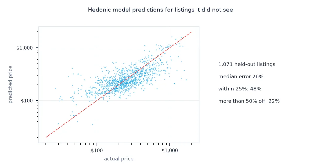
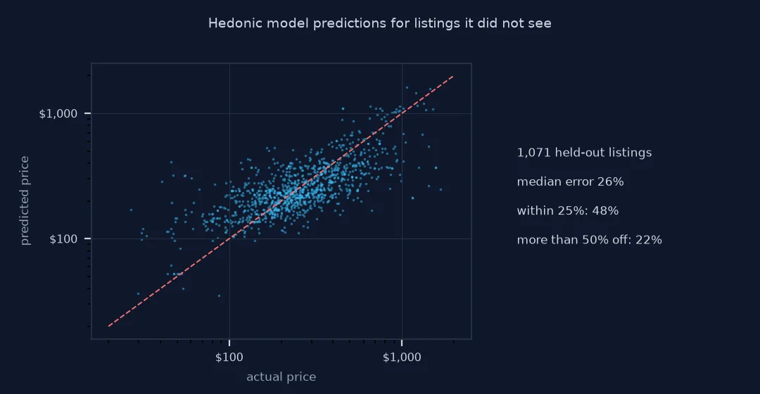
held-out listings: 1,071; median absolute error 26% of the price; within 25%: 48%

On 1,071 listings the model never saw, the typical error is 26% of the price, and 48% of predictions are within 25%. That is useful for ranking and for explaining prices, and too rough to price an individual listing.

The price of a room type

The data used on this page

The Inside Airbnb listings for Washington, D.C. from the snapshot of 24 June 2026 (CC BY 4.0), with prices between $20 and $2,000 a night and the number of bathrooms parsed from bathrooms_text where needed.

from pathlib import Path

import numpy as np
import pandas as pd
import requests

Path("data").mkdir(exist_ok=True)
BASE = "https://data.insideairbnb.com/united-states/dc/washington-dc/2026-06-24"
p = Path("data/listings.csv.gz")
if not p.exists():
    r = requests.get(f"{BASE}/data/listings.csv.gz", timeout=600); r.raise_for_status(); p.write_bytes(r.content)
L = pd.read_csv(p)
L["price_usd"] = pd.to_numeric(L.price.str.replace(r"[$,]", "", regex=True), errors="coerce")
L["bathrooms"] = L.bathrooms.fillna(pd.to_numeric(L.bathrooms_text.str.extract(r"([\d.]+)")[0], errors="coerce"))
D = L[L.price_usd.between(20, 2000)].dropna(subset=["bedrooms", "bathrooms", "accommodates"]).copy()
D["log_price"] = np.log(D.price_usd)
D["long_stay"] = (D.minimum_nights >= 30).astype(int)
print(f"listings: {len(L):,}; used in the model: {len(D):,}")

listings: 6,945; used in the model: 5,126

5,126 of the 6,945 listings have a price between $20 and $2,000 and complete size fields.

Example 1: the price of a room type

The room-type coefficients compare each type with the reference, entire homes:

rt = m2.params.filter(like="room_type")
print({k.split("T.")[1].rstrip("]"): f"{pct(v):+.0f}%" for k, v in rt.items()})

{'Hotel room': '+2%', 'Private room': '-11%', 'Shared room': '-80%'}

Compared with entire homes of the same size and neighbourhood, private rooms are 11% cheaper and shared rooms 80% cheaper, while hotel rooms are about the same.

Horizontal bars of neighbourhood effects relative to the reference area, six lowest and six highest — Neighbourhood effects run from -22% to +163% for the same size and room type.

Implicit prices of characteristics

Scatter of predicted against actual price for 1,071 held-out listings on log axes — Median error 26%; 48% of predictions are within 25%.

A hedonic model treats a price as the sum of the implicit prices of a good's characteristics. It is estimated by regressing price, usually its logarithm, on those characteristics. With log price, a coefficient b means each unit of the variable multiplies the price by e^b, so coefficients read as percentage effects, which suits prices where a bedroom adds more in an expensive area than in a cheap one. Categorical variables such as room type or neighbourhood enter as sets of dummy variables relative to a reference category, which is why each coefficient is "compared with entire homes" or "compared with the reference area".

Two habits make the coefficients trustworthy. Location must be in the model, because it is correlated with almost every other characteristic: central listings are smaller and pricier, so a model without location mixes size and place. Fixed effects for neighbourhoods are the simplest way, distance to the centre or to transit another. And a model should be checked on data it was not fitted on. The R² measures fit, but the held-out error is what a user of the model's predictions experiences. Hedonic coefficients describe associations in the data, not causal effects: superhost status, for instance, may reflect quality the model does not see.

Retransformation, heteroskedasticity and autocorrelation

Held-out testing is what turns a fit into a prediction.

Retransformation: exp of a predicted log price estimates the median, not the mean; a smearing correction recovers the mean.
Heteroskedasticity: use robust standard errors (fit(cov_type="HC3")) for valid confidence intervals.
Spatial autocorrelation: residuals of nearby listings are correlated; spatial models or clustered errors account for it.
Amenities: the amenities column is a JSON list; dummies for pools, parking or workspaces add explanatory power.

Internal links

How to measure Airbnb prices against distance to transit in Python — location as distance
House price index methods explained — hedonic indices in context
How to analyse Inside Airbnb listings in Python — the data

FAQ

What is a hedonic price model?

A regression that explains a price by the characteristics of the good, giving each characteristic an implicit price.

Why use log price in a hedonic regression?

Effects are proportional and prices are skewed; log price gives percentage effects and better-behaved residuals.

How do I include location in a price model?

Add neighbourhood fixed effects with C(neighbourhood), or continuous measures such as distance to the centre.

How accurate are hedonic price predictions?

Check on held-out listings; for D.C. Airbnb prices, a basic model's typical error is a sizeable share of the price.