Fixing House Price Averages Skewed by Outliers

Problem statement

The average house price you calculate comes out well above the figures you have seen reported, and for a small area it jumps when a single sale is added or removed. House prices are skewed. Most sales cluster around a typical value, a long tail runs up to tens of millions, and transactions that are not ordinary home sales, such as portfolio and company purchases, sit in the same files. A mean is pulled toward that tail. The median, a trimmed mean or a geometric mean describe the typical sale far better, and removing non-standard transactions matters as much as the choice of statistic.

This page shows the effect on the 2024 HM Land Registry Price Paid file. It compares the mean and the median with and without category B transactions, measures how much the top 0.1% of sales moves each statistic, and compares robust alternatives by district.

Quick answer

Use the median of standard (category A) sales:

A = P[P.ppd_category == "A"]
print(f"all transactions: mean £{P.price.mean():,.0f}, median £{P.price.median():,.0f}")
print(f"standard sales only: mean £{A.price.mean():,.0f}, median £{A.price.median():,.0f}")

all transactions: mean £400,202, median £280,000
standard sales only: mean £369,875, median £291,000

Across all 931,453 transactions the mean is £400,202, 43% above the median of £280,000. Dropping category B lowers the mean to £369,875 and raises the median to £291,000, because category B holds both the largest prices and many cheaper non-standard sales.

How the top end moves each statistic, robust alternatives, districts

1. How much the top end moves each statistic

cut = A.price.quantile(0.999)
trim = A[A.price <= cut]
print(f"top 0.1% of standard sales: above £{cut:,.0f}; removing them changes the mean by {trim.price.mean() / A.price.mean() - 1:+.1%} and the median by {trim.price.median() / A.price.median() - 1:+.2%}")
print(f"share of the total value of standard sales in the top 1%: {A.price.nlargest(len(A) // 100).sum() / A.price.sum():.1%}")

top 0.1% of standard sales: above £4,200,000; removing them changes the mean by -1.9% and the median by -0.34%
share of the total value of standard sales in the top 1%: 7.4%

The top 0.1% of standard sales, those above £4.2 million, move the mean by 1.9% and the median by 0.34%. The top 1% of sales account for 7.4% of all the money spent.

2. Robust alternatives

from scipy.stats import trim_mean
print(f"median £{A.price.median():,.0f}; 10% trimmed mean £{trim_mean(A.price, 0.1):,.0f}; geometric mean £{np.exp(np.log(A.price).mean()):,.0f}; mean £{A.price.mean():,.0f}")

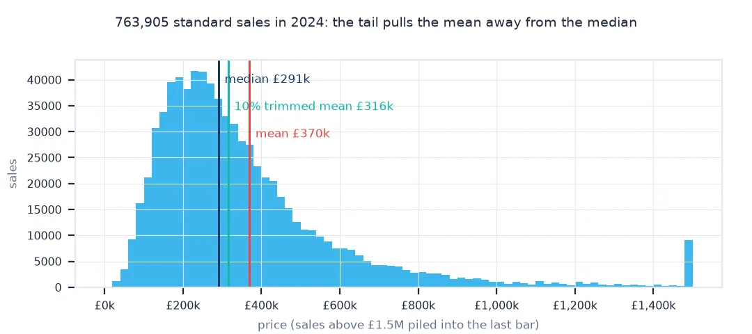
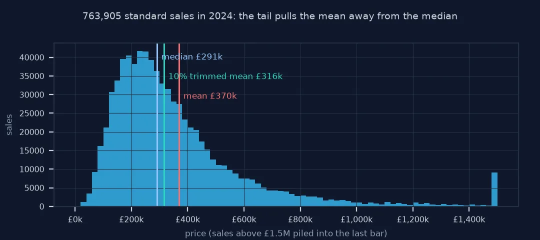
median £291,000; 10% trimmed mean £315,836; geometric mean £295,253; mean £369,875

The robust measures sit close together, between the median of £291,000 and the trimmed mean of £315,836, while the mean is £369,875.

3. The effect by district

Small districts are most affected by single sales. Compare mean and median for each district:

d = A.groupby("district").price.agg(["size", "mean", "median"])
d["ratio"] = d["mean"] / d["median"]
print(f"districts: {len(d)}; mean-to-median ratio: median {d.ratio.median():.2f}, largest {d.ratio.max():.2f} ({d.ratio.idxmax().title()})")
print(f"districts where the mean is more than 30% above the median: {(d.ratio > 1.3).sum()}")

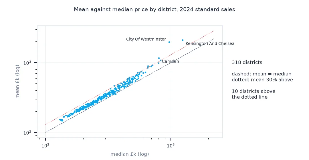
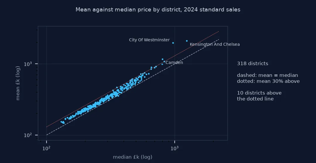
districts: 318; mean-to-median ratio: median 1.14, largest 2.03 (City Of Westminster)
districts where the mean is more than 30% above the median: 10

In a typical district the mean is 14% above the median. In the City of Westminster it is more than double, and in 10 districts the mean exceeds the median by more than 30%, so ranking districts by mean and by median gives different orders.

The shape of the price distribution

The data used on this page

HM Land Registry Price Paid Data for 2024 (© Crown copyright 2026, Open Government Licence v3.0), all categories.

from pathlib import Path

import numpy as np
import pandas as pd
import requests

Path("data").mkdir(exist_ok=True)
CSV = Path("data/pp-2024.csv")
if not CSV.exists():
    r = requests.get("http://prod1.publicdata.landregistry.gov.uk.s3-website-eu-west-1.amazonaws.com/pp-2024.csv", timeout=1800); r.raise_for_status(); CSV.write_bytes(r.content)
COLS = ["transaction_id", "price", "date", "postcode", "property_type", "old_new", "duration", "paon", "saon",
        "street", "locality", "town", "district", "county", "ppd_category", "record_status"]
P = pd.read_csv(CSV, header=None, names=COLS, usecols=["price", "property_type", "district", "ppd_category"])
print(f"{len(P):,} transactions; largest £{P.price.max():,.0f}, smallest £{P.price.min():,.0f}")

931,453 transactions; largest £180,000,000, smallest £1

The 2024 file runs from £1 to £180,000,000.

Example 1: the shape of the distribution

The skew shows in the quantiles:

q = A.price.quantile([0.01, 0.1, 0.25, 0.5, 0.75, 0.9, 0.99, 0.999])
print({f"{int(k * 1000) / 10}%": f"£{v:,.0f}" for k, v in q.items()})
print(f"skewness of prices {A.price.skew():.1f}; of log prices {np.log(A.price).skew():.2f}")

{'1.0%': '£67,000', '10.0%': '£135,000', '25.0%': '£195,000', '50.0%': '£291,000', '75.0%': '£432,000', '90.0%': '£642,500', '99.0%': '£1,585,000', '99.9%': '£4,200,000'}
skewness of prices 27.9; of log prices 0.23

Half of standard sales are between £195,000 and £432,000, but the top 1% start at £1,585,000. The skewness of 27.9 falls to 0.23 on log prices, which is why logs are the usual scale for modelling prices.

A heavy upper tail

House prices follow roughly a log-normal distribution with a heavy upper tail. Most homes sell within a few hundred thousand pounds of the typical price, while a small number sell for millions, and in a national file for tens of millions. The arithmetic mean gives each pound equal weight, so those few sales pull it well above what a typical buyer pays, and it moves noticeably when a single very large sale is added or removed, especially in small areas. The median is unaffected by how large the largest values are, which is why official statistics, including the UK House Price Index, report medians or use methods built on log prices.

The data's own structure adds a second layer. Category B transactions in Price Paid Data include transfers to companies, buy-to-let purchases identified by a mortgage, repossessions and other sales at prices that do not reflect a single home on the open market, and they include the largest prices in the file. Filtering to category A removes them before any statistic is computed. When a mean is needed, for example to add values up, a trimmed mean or the mean of log prices (the geometric mean) gives a stable alternative, as long as the method is stated.

Totals, logs and low outliers

• Totals: if the question is total value of sales, the mean is the right statistic; the problem is only using it as "typical".
• Logs for models: regressions on log price treat proportional differences evenly and reduce the influence of the tail.
• Small areas: with under a few hundred sales, even the median moves with the mix; report the count.
• Low outliers: very low prices (a few thousand pounds) are often part-shares or errors; check the bottom tail too.

Internal links

• How to analyse HM Land Registry price paid data in Python — the data
• How to find the most expensive streets in England and Wales with Python — medians in rankings
• Price paid data explained — what category B contains

FAQ

Why is the average house price so high?

The mean is pulled up by a few very expensive sales; the median describes a typical home.

Should I use mean or median for house prices?

The median for typical prices; the mean only when you need totals.

What is category B in Land Registry data?

Additional transactions such as company purchases, buy-to-let sales identified by a mortgage and repossessions; exclude them for typical prices.

What is a trimmed mean?

The mean after removing a fixed share of the highest and lowest values, for example 10% at each end.