
How to Measure Airbnb Prices Against Distance to Transit in Python
On this page
Problem statement
Location is the first thing guests pay for, and in a city with a metro system, distance to the nearest station is one of the clearest measures of location. Testing that in data takes a join between two sources: listing coordinates from Inside Airbnb and station locations from OpenStreetMap, measured in a projected CRS, then binned and compared like for like, since the listings near downtown stations are also different kinds of listing.
This page computes the distance from every entire-home listing in the Inside Airbnb snapshot of Washington, D.C. of 24 June 2026 to the nearest Metro station in OpenStreetMap. It compares median prices by distance band, controls for size, and fits a simple regression of log price on distance.
Quick answer
Project both layers to UTM, find each listing's nearest station with a spatial index, and bin the distances:
E0 = L[(L.room_type == "Entire home/apt") & L.price_usd.notna()]
E = gpd.GeoDataFrame(E0, geometry=gpd.points_from_xy(E0.longitude, E0.latitude), crs=4326).to_crs(32618)
near = gpd.sjoin_nearest(E, S[["name", "geometry"]].rename(columns={"name": "station"}), how="left", distance_col="dist_m")
near = near[~near.index.duplicated()]
near["band"] = pd.cut(near.dist_m, [0, 400, 800, 1600, 20000], labels=["<400 m", "400-800 m", "0.8-1.6 km", ">1.6 km"])
print(f"entire homes: {len(near):,}; median distance to a Metro station {near.dist_m.median():.0f} m")
print(near.groupby("band", observed=True).agg(listings=("id", "size"), median_price=("price_usd", "median")).round(0).to_string())
entire homes: 4,618; median distance to a Metro station 729 m
listings median_price
band
<400 m 981 258.0
400-800 m 1554 243.0
0.8-1.6 km 1607 217.0
>1.6 km 476 209.0
The 4,618 priced entire homes are a median 729 m from the nearest Metro station. Prices fall with distance, from a median of $258 within 400 m to $209 beyond 1.6 km.
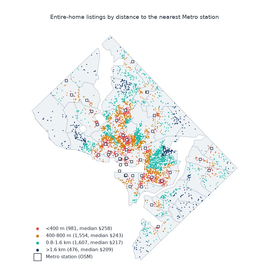
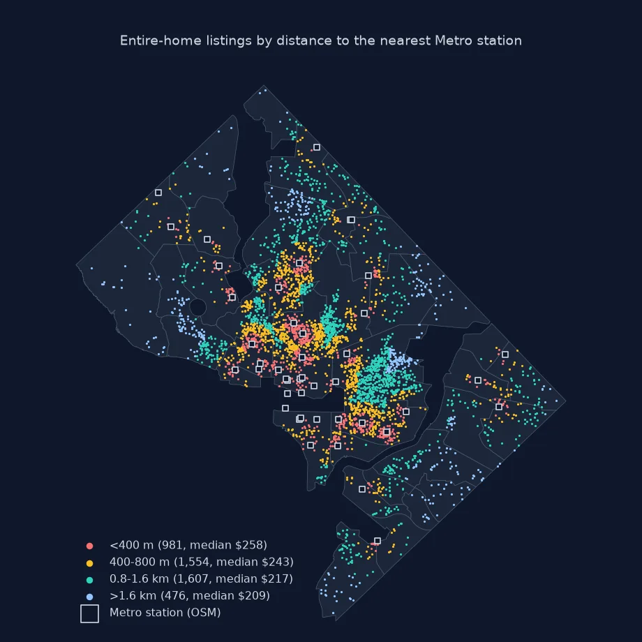
Like with like, a simple regression, stations with most listings
1. Compare like with like
Larger homes are farther from the centre. Compare price per guest:
near["per_guest"] = near.price_usd / near.accommodates.clip(lower=1)
print(near.groupby("band", observed=True).agg(median_accommodates=("accommodates", "median"), price_per_guest=("per_guest", "median")).round(1).to_string())
median_accommodates price_per_guest
band
<400 m 4.0 72.9
400-800 m 4.0 64.2
0.8-1.6 km 4.0 55.2
>1.6 km 4.0 53.2
Homes in every band sleep a median of four, so size does not explain the gradient here. Price per guest falls from $72.90 within 400 m to $53.20 beyond 1.6 km.
2. A simple regression
Fit log price on distance and size, so the coefficient reads as a percentage change:
import statsmodels.formula.api as smf
d = near.assign(log_price=np.log(near.price_usd), km=near.dist_m / 1000, bedrooms=near.bedrooms.fillna(1)).query("price_usd > 20 and price_usd < 2000")
m = smf.ols("log_price ~ km + bedrooms + accommodates", data=d).fit()
print(f"n = {int(m.nobs)}; R² = {m.rsquared:.2f}; each km farther from a station: {100 * (np.exp(m.params['km']) - 1):+.1f}% price (95% CI {100 * (np.exp(m.conf_int().loc['km', 0]) - 1):+.1f} to {100 * (np.exp(m.conf_int().loc['km', 1]) - 1):+.1f}%)")
n = 4598; R² = 0.33; each km farther from a station: -19.1% price (95% CI -21.2 to -16.9%)
Controlling for bedrooms and capacity, each kilometre from a station is associated with a 19.1% lower price, with a 95% interval of 16.9% to 21.2%, over 4,598 listings.
3. Which stations have the most listings nearby
top = near[near.dist_m <= 800].groupby("station").agg(listings=("id", "size"), median_price=("price_usd", "median")).sort_values("listings", ascending=False)
print(top.head(5).round(0).to_string())
listings median_price
station
Dupont Circle 289 216.0
Shaw–Howard University 230 290.0
NoMa–Gallaudet U 220 299.0
Eastern Market 201 232.0
Georgia Avenue–Petworth 177 195.0
Dupont Circle has the most entire homes within 800 m, 289, followed by Shaw-Howard University, NoMa-Gallaudet, Eastern Market and Georgia Avenue-Petworth. Median prices around them range from $195 to $299.
The price gradient in numbers
The data used on this page
The Inside Airbnb snapshot for Washington, D.C. dated 24 June 2026 (CC BY 4.0), and Metro stations (railway=station, station=subway) from the Geofabrik OpenStreetMap extract for D.C. of 1 January 2026 (© OpenStreetMap contributors, ODbL), read with pyosmium.
from pathlib import Path

import geopandas as gpd
import numpy as np
import osmium
import pandas as pd
import requests

Path("data").mkdir(exist_ok=True)
BASE = "https://data.insideairbnb.com/united-states/dc/washington-dc/2026-06-24"
def cached(path, url):
    p = Path(path)
    if not p.exists():
        r = requests.get(url, timeout=600); r.raise_for_status(); p.write_bytes(r.content)
    return p
L = pd.read_csv(cached("data/listings.csv.gz", f"{BASE}/data/listings.csv.gz"))
L["price_usd"] = pd.to_numeric(L.price.str.replace(r"[$,]", "", regex=True), errors="coerce")
PBF = cached("data/district-of-columbia-260101.osm.pbf", "https://download.geofabrik.de/north-america/us/district-of-columbia-260101.osm.pbf")
fp = (osmium.FileProcessor(str(PBF)).with_areas().with_filter(osmium.filter.EntityFilter(osmium.osm.NODE | osmium.osm.AREA))
      .with_filter(osmium.filter.TagFilter(("railway", "station"))).with_filter(osmium.filter.GeoInterfaceFilter(tags=["name", "station"])))
S = gpd.GeoDataFrame.from_features(fp, crs=4326)
S = S[S.station == "subway"].to_crs(32618)
S["geometry"] = S.representative_point()
print(f"{len(L):,} listings; {len(S)} Metro station features in the extract (D.C. and its margin)")
6,945 listings; 44 Metro station features in the extract (D.C. and its margin)
The OSM extract yields 44 Metro station features, in the District and its margin.
Example 1: the price gradient in numbers
The ratio of the median price within 400 m of a station to the median beyond 1.6 km:
b = near.groupby("band", observed=True).price_usd.median()
print(f"median within 400 m ${b['<400 m']:.0f}; beyond 1.6 km ${b['>1.6 km']:.0f}; ratio {b['<400 m'] / b['>1.6 km']:.2f}")
median within 400 m $258; beyond 1.6 km $209; ratio 1.23
The median within 400 m of a station is 23% above the median beyond 1.6 km.
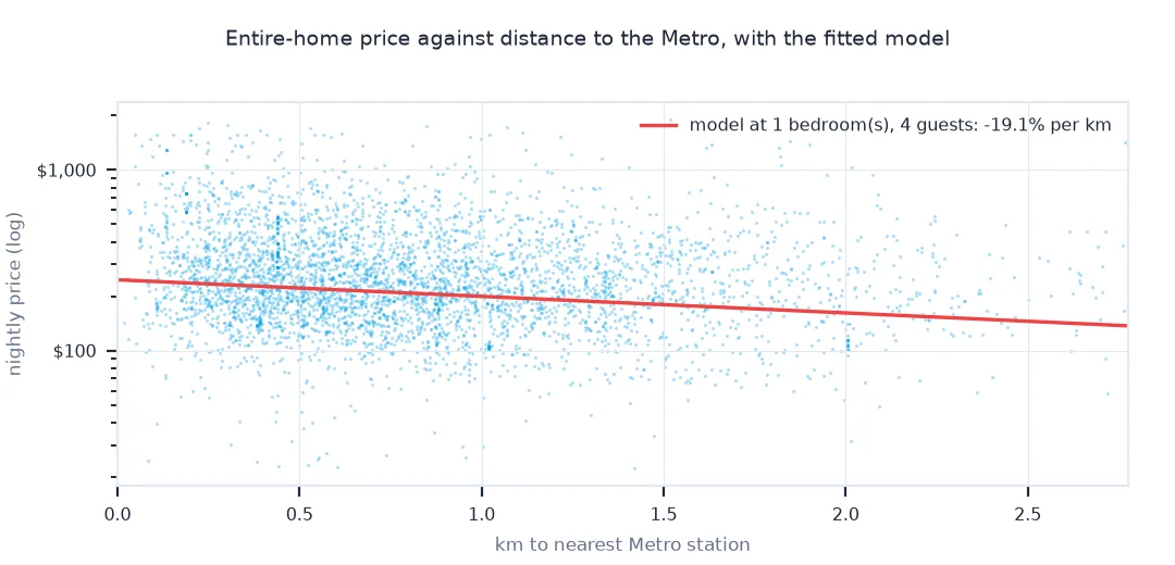
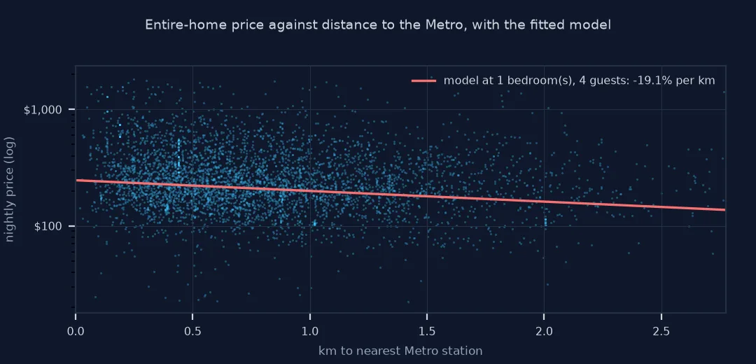
Transit distance as a bundle of things guests value
Distance to transit is a standard variable in housing economics, and for short-term rentals it stands in for a bundle of things guests value: easy access to sights, restaurants and offices, and a central location in general. Computing it needs both layers in a projected CRS, so distances are in metres, and a nearest-neighbour search, which GeoPandas' sjoin_nearest performs with a spatial index. Station locations come from OpenStreetMap, reduced to one point per station, and include stations just outside the city so listings near the border find their true nearest station.
The raw gradient overstates the effect of the station itself. Listings near downtown stations are smaller apartments in denser, more expensive areas, while those far from stations are often larger houses. Comparing price per guest, or controlling for bedrooms and capacity in a regression, separates some of that. Even then, distance to a station is correlated with everything else about a central location, so the coefficient describes how prices vary across the city, not what building a new station would do. Inside Airbnb's location blurring, up to about 150 m, adds noise to distances under a few hundred metres.
Walking distance, entrances and log prices
- Straight-line vs walking distance: network distance along streets is more realistic; OSMnx can compute it for a sample.
- Station entrances: large stations have several entrances; the station point is an approximation.
- Log prices: model log price so effects read as percentages and the skew does not dominate.
- Outliers: trim implausible prices before regression; the result depends on the trimming rule, so state it.
Internal links
- How to get railway lines and stations from OpenStreetMap in Python — the stations
- How to build a hedonic price model for Airbnb listings in Python — more variables
- How to find all points within a radius in Python — distance queries
FAQ
How do I calculate the distance from Airbnb listings to the nearest station?
Project listings and stations to a metric CRS and use gpd.sjoin_nearest(listings, stations, distance_col="dist_m").
Are Airbnb listings near metro stations more expensive?
In D.C. the median entire home within 400 m of a Metro station costs more than one beyond 3.2 km; part of that difference is size and central location, not the station itself.
Why use log price in a regression?
Prices are skewed and effects are roughly proportional, so log price gives percentage effects and better-behaved residuals.
Where do I get metro station locations?
From OpenStreetMap (railway=station with station=subway), or from the transit agency's GTFS feed.