Fixing a Gutenberg-Richter b-Value That Comes Out Too Low

Problem statement

A b-value of 0.7 for a region where every study finds about 1.0 is almost never a discovery. The usual cause is that the cut-off magnitude is below the magnitude of completeness for part of the catalogue, so small earthquakes are missing, the frequency-magnitude distribution flattens, and the maximum-likelihood estimate follows it down. It is easy to miss because completeness is not one number: after a large earthquake the network misses small events for days, so a cut-off that is right for the catalogue as a whole is far too low for the first hours of an aftershock sequence.

This page takes the first six months of the 2019 Ridgecrest, California, sequence from the USGS catalogue, shows how a single cut-off gives a b-value that is too low, measures how completeness changed over time, and gets a consistent b-value by using a cut-off that holds for every period.

Quick answer

Estimate the magnitude of completeness per period, and use a cut-off at or above the largest one:

mc_all = round(m.value_counts().idxmax() + 0.2, 1)
print(f"one Mc for the whole catalogue: M{mc_all:.1f}; b = {b_mle(m, mc_all)[0]:.3f}")
for name, part in periods.items():
    mp = part.mag.round(1)
    mc_p = round(mp.value_counts().idxmax() + 0.2, 1)
    print(f"{name:>15}: {len(part):>6,} events, Mc M{mc_p:.1f}; b at M{mc_all:.1f} = {b_mle(mp, mc_all)[0]:.3f}, at its own Mc = {b_mle(mp, mc_p)[0]:.3f}")

one Mc for the whole catalogue: M1.2; b = 0.700
      first day:  3,501 events, Mc M2.2; b at M1.2 = 0.365, at its own Mc = 0.642
    days 1 to 7:  9,141 events, Mc M1.6; b at M1.2 = 0.763, at its own Mc = 0.927
   after a week: 28,790 events, Mc M1.2; b at M1.2 = 0.936, at its own Mc = 0.936

Maximum curvature over the whole catalogue gives Mc = M1.2 and a b-value of 0.700, far below the value near 1 that almost every region shows (see estimating b and completeness). Split by period, the cause is plain. In the first day after the mainshock Mc is M2.2, and a cut-off of M1.2 gives b = 0.365; in days 1 to 7 Mc is M1.6. Only after a week is M1.2 complete, and there b = 0.936 with either cut-off.

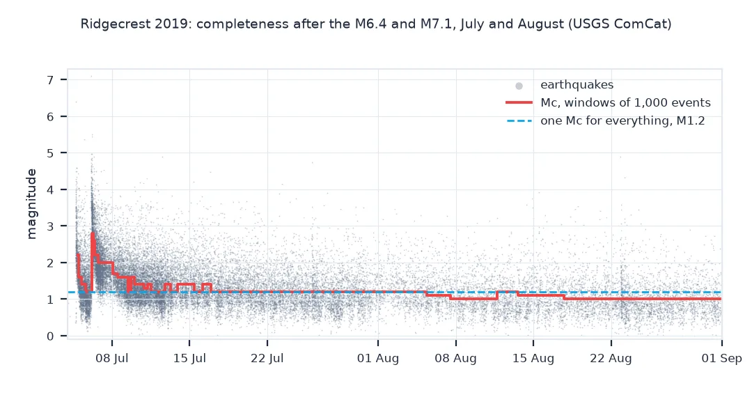
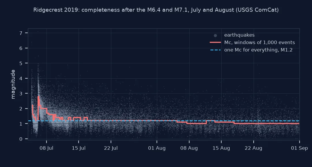
Completeness over time, moving-window Mc, one safe cut-off

1. See completeness change with time

Plot or tabulate the smallest magnitudes recorded in each window. Right after the mainshock, small events vanish from the catalogue because they are buried in the waves of larger ones:

q = cat.set_index("time").mag
for start, end in (("2019-07-06 03:19", "2019-07-06 06:00"), ("2019-07-06 06:00", "2019-07-07"), ("2019-07-07", "2019-07-10"),
                   ("2019-07-10", "2019-08-01"), ("2019-08-01", "2020-01-01")):
    w = q[start:end].round(1)
    print(f"{start[:16]} to {end[:10]}: {len(w):>6,} events; most common magnitude M{w.value_counts().idxmax():.1f}; 5th percentile M{w.quantile(0.05):.2f}")

2019-07-06 03:19 to 2019-07-06:    548 events; most common magnitude M3.4; 5th percentile M2.50
2019-07-06 06:00 to 2019-07-07:  4,103 events; most common magnitude M1.8; 5th percentile M1.30
2019-07-07 to 2019-07-10:  6,318 events; most common magnitude M1.4; 5th percentile M0.90
2019-07-10 to 2019-08-01: 14,807 events; most common magnitude M1.0; 5th percentile M0.60
2019-08-01 to 2020-01-01: 19,088 events; most common magnitude M0.8; 5th percentile M0.30

In the first three hours after the mainshock the most common recorded magnitude was M3.4 and only 5% of the 548 events were below M2.5. By the rest of that day the most common magnitude was M1.8; between 10 and 31 July, M1.0; and from August, M0.8. The network had not changed; the small events were there all along, hidden in the shaking from larger ones.

2. Estimate Mc in moving windows

Moving windows of a fixed number of events follow completeness as it changes. Take windows of 1,000 events stepping by 500:

mags, times = cat.mag.round(1).values, cat.time.values
rows = []
for i in range(0, len(cat) - 1000, 500):
    w = pd.Series(mags[i:i + 1000])
    rows.append((times[i + 500], round(w.value_counts().idxmax() + 0.2, 1)))
mcw = pd.DataFrame(rows, columns=["time", "mc"]).set_index("time").mc
print(f"windows: {len(mcw)}; Mc from M{mcw.min():.1f} to M{mcw.max():.1f}")
print(f"first window, centred {mcw.index[0]:%d %b %H:%M}: M{mcw.iloc[0]:.1f}; Mc back to M{mcw.iloc[-1]:.1f} or below from {mcw[mcw <= mcw.iloc[-1]].index[0]:%d %b}")

windows: 88; Mc from M0.8 to M2.8
first window, centred 04 Jul 21:40: M2.2; Mc back to M1.0 or below from 08 Aug

Across 88 windows of 1,000 events, Mc ranges from M2.8 to M0.8. The first window, centred on 21:40 UTC on 4 July, four hours after the M6.4 foreshock at 17:33, is already at M2.2. Mc first came back down to M1.0 on 8 August, a month after the mainshock, and still rose to M1.1 or M1.2 for a few windows after that, as later bursts of aftershocks arrived.

3. One cut-off that holds everywhere

For a b-value of the whole sequence, choose a cut-off at or above every window's Mc, or drop the incomplete start:

safe = mcw.max()
after = cat[cat.time >= "2019-07-07"].mag.round(1)
print(f"cut-off M{safe:.1f}, all events: b = {b_mle(m, safe)[0]:.3f} ± {b_mle(m, safe)[2]:.3f} ({b_mle(m, safe)[1]:,} events)")
mc_after = round(after.value_counts().idxmax() + 0.2, 1)
print(f"from 7 July only, Mc M{mc_after:.1f}: b = {b_mle(after, mc_after)[0]:.3f} ± {b_mle(after, mc_after)[2]:.3f} ({b_mle(after, mc_after)[1]:,} events)")

cut-off M2.8, all events: b = 0.840 ± 0.018 (1,619 events)
from 7 July only, Mc M1.2: b = 0.855 ± 0.006 (18,276 events)

A cut-off of M2.8 is complete in every window and gives b = 0.840 ± 0.018 from 1,619 events. Dropping the first three days instead and taking maximum curvature again gives Mc = M1.2 and b = 0.855, but the moving windows show M1.2 is still too low for 7 to 10 July, so that estimate is pulled down too. The 0.840 at M2.8 and the 0.936 for the period after a week do not agree within their errors either: b also varies with the magnitude range and the period it describes. Report the cut-off and the period with every b-value.

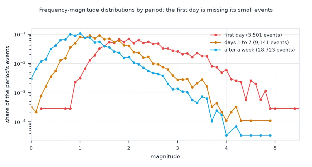
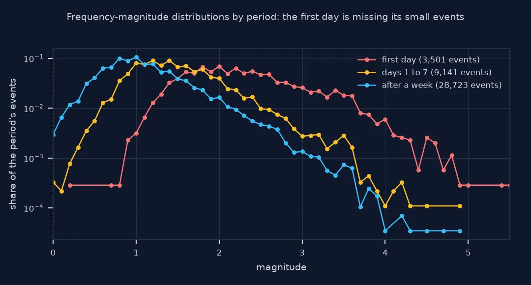
The distribution in each period

The data used on this page

Every event of magnitude 0 or more between 35.4° and 36.1°N and 118.0° and 117.2°W from 4 July to 31 December 2019 in the USGS ComCat catalogue, from the FDSN event service. The sequence began with an M6.4 foreshock on 4 July and the M7.1 mainshock on 6 July. The service returns at most 20,000 events per request, so the setup asks for one week at a time.

import io
import zipfile
from pathlib import Path

import numpy as np
import pandas as pd
import requests

Path("data").mkdir(exist_ok=True)
# the 26 weekly files as ComCat served them on 9 October 2026 (reviews keep revising the catalogue);
# week() below queries live for any file that is missing, so delete data/ to download afresh
if not Path("data/ridgecrest_m0_20190704.csv").exists():
    reply = requests.get("https://data.spatialworkflow.io/comcat-ridgecrest-2019-m0-2026-10-09.zip", timeout=300)
    reply.raise_for_status()
    with zipfile.ZipFile(io.BytesIO(reply.content)) as archive:
        archive.extractall("data")
Q = "https://earthquake.usgs.gov/fdsnws/event/1/query"
BOX = dict(minlatitude=35.4, maxlatitude=36.1, minlongitude=-118.0, maxlongitude=-117.2)
def week(t0):
    t1 = t0 + pd.Timedelta(days=7)
    p = Path(f"data/ridgecrest_m0_{t0:%Y%m%d}.csv")
    if not p.exists():
        r = requests.get(Q, params=dict(format="csv", starttime=f"{t0:%Y-%m-%d}", endtime=f"{min(t1, pd.Timestamp('2020-01-01')):%Y-%m-%d}",
                                        minmagnitude=0, orderby="time-asc", **BOX), timeout=600)
        r.raise_for_status()
        p.write_text(r.text)
    d = pd.read_csv(p)
    assert len(d) < 20000, f"{t0:%Y-%m-%d}: {len(d)} rows, at the cap"
    return d
def b_mle(mags, mc, dm=0.1):
    x = mags[mags >= mc - 1e-9]
    b = np.log10(np.e) / (x.mean() - (mc - dm / 2))
    return b, len(x), 2.3 * b ** 2 * np.sqrt(((x - x.mean()) ** 2).sum() / (len(x) * (len(x) - 1)))
raw = pd.concat([week(t) for t in pd.date_range("2019-07-04", "2019-12-31", freq="7D")], ignore_index=True)
cat = raw[raw["type"] == "earthquake"].drop_duplicates("id").copy()
cat["time"] = pd.to_datetime(cat.time).dt.tz_localize(None)
cat = cat.sort_values("time").reset_index(drop=True)
m = cat.mag.round(1)
main = cat.loc[cat.mag.idxmax()]
periods = {"first day": cat[(cat.time >= main.time) & (cat.time < main.time + pd.Timedelta(days=1))],
           "days 1 to 7": cat[(cat.time >= main.time + pd.Timedelta(days=1)) & (cat.time < main.time + pd.Timedelta(days=7))],
           "after a week": cat[cat.time >= main.time + pd.Timedelta(days=7)]}
print(f"{len(cat):,} earthquakes; largest M{main.mag} at {main.time:%Y-%m-%d %H:%M} UTC")

44,935 earthquakes; largest M7.1 at 2019-07-06 03:19 UTC

The six months hold 44,935 earthquakes. The largest is the M7.1 mainshock at 03:19 UTC on 6 July 2019.

Example 1: the frequency-magnitude distribution of each period

Compare the shape of the distribution in the first day with that after a week, normalised to the same total:

for name in ("first day", "after a week"):
    c = periods[name].mag.round(1).value_counts(normalize=True).sort_index()
    print(f"{name:>13}: share at M0.5-0.9 {c.loc[0.5:0.9].sum():.1%}, M1.0-1.9 {c.loc[1.0:1.9].sum():.1%}, M2.0+ {c.loc[2.0:].sum():.1%}")

    first day: share at M0.5-0.9 0.3%, M1.0-1.9 33.7%, M2.0+ 66.0%
 after a week: share at M0.5-0.9 35.8%, M1.0-1.9 50.3%, M2.0+ 7.2%

Normalised to the same total, the first day's catalogue has almost nothing below M1.0, 0.3%, and two-thirds of its events at M2.0 or more. After a week, 35.8% are between M0.5 and M0.9 and only 7.2% are M2.0 or more. Fitted at one cut-off, the first distribution is far flatter, which is all a low b-value is.

Missing small events lower b

The maximum-likelihood b-value assumes that, above the cut-off, every earthquake is in the catalogue. Below completeness the smallest bins are depleted, the mean magnitude of the kept events rises, and because b is inversely proportional to the mean magnitude minus the cut-off, the estimate falls. A cut-off a few tenths of a magnitude too low is enough to take b from 1.0 to 0.8, a difference that would be scientifically interesting if it were real.

Completeness changes with time for two reasons. Over years, networks add stations and Mc falls. Over hours, a large earthquake and its biggest aftershocks shake every station for minutes, and the many small aftershocks in that time are not detected or not located. A catalogue that covers an aftershock sequence therefore needs either a time-varying Mc, or a single cut-off high enough for its worst period, or the earliest hours left out.

Event windows and maximum curvature

• Moving windows of events, not of time: a fixed number of events per window gives the estimate a constant sample size; windows of fixed duration hold thousands of events early on and a handful later.
• Maximum curvature underestimates: the +0.2 correction is a rule of thumb; methods based on goodness of fit or b-value stability give more robust Mc estimates.
• Magnitude types: a switch from local to moment magnitude at some size also bends the distribution, independently of completeness.
• Declustering: removing aftershocks also removes the period of worst completeness, but changes which events b describes.

Internal links

• How to estimate b-value and completeness in Python
• Earthquake catalogues explained: magnitudes, completeness and declustering — completeness in general
• Earthquake counts rise over time in my catalogue — completeness changing over years

FAQ

Why is my b-value lower than expected?

Most often the cut-off magnitude is below the magnitude of completeness for some of the catalogue, typically the first hours or days after a large earthquake; small events are missing and the estimate falls.

How do I find the magnitude of completeness over time?

Estimate it in moving windows of a fixed number of events, for example 1,000, and plot it against the time of each window.

Can I just raise the cut-off?

Yes: a cut-off at or above the highest Mc of every period is valid for the whole catalogue, at the cost of fewer events.

Is a low b-value after a big earthquake real?

It can be, but check completeness first; an apparent low b in the first days of a sequence is usually missing small events.