Cartograms Explained: Trading Geography for Size

On this page

Problem statement

Every map trades something. An ordinary map keeps area true to land and gives the most visual weight to the largest, often emptiest, regions. A cartogram changes the rule: each region's area becomes proportional to something else — population, votes, income, cases — and the geography bends to fit. There are several ways to bend it. Each keeps some properties of the original map and gives others up, and choosing between them is a matter of knowing which property your readers need.

This page puts the four main families — contiguous, Dorling, non-contiguous (Olson) and the plain equal-area map they start from — side by side on one dataset, the 2024 presidential vote by state. It measures what each keeps: how accurately area follows the votes, how many real borders survive, and how much the shapes change.

Quick answer

Score every method on the same three questions: does area follow the value, are neighbours still neighbours, and are the shapes still recognisable?

rows = []
for name, geoms in METHODS.items():
    a = shapely.area(np.array(geoms, dtype=object))
    err = np.abs(a / a.sum() - VOTE_SHARE).sum() / 2                      # share of the map in the wrong place
    rows.append({"method": name, "area misallocated": f"{err:.0%}",
                 "real borders kept": f"{len(touching(geoms) & REAL) / len(REAL):.0%}",
                 "median shape kept": f"{np.median(compactness(geoms) / BASE_SHAPE):.2f}" if name != "Dorling" else "circles"})
print(pd.DataFrame(rows).to_string(index=False))

        method area misallocated real borders kept median shape kept
equal-area map               38%              100%              1.00
    contiguous                0%              100%              0.76
       Dorling                0%               17%           circles
         Olson                0%                3%              1.00

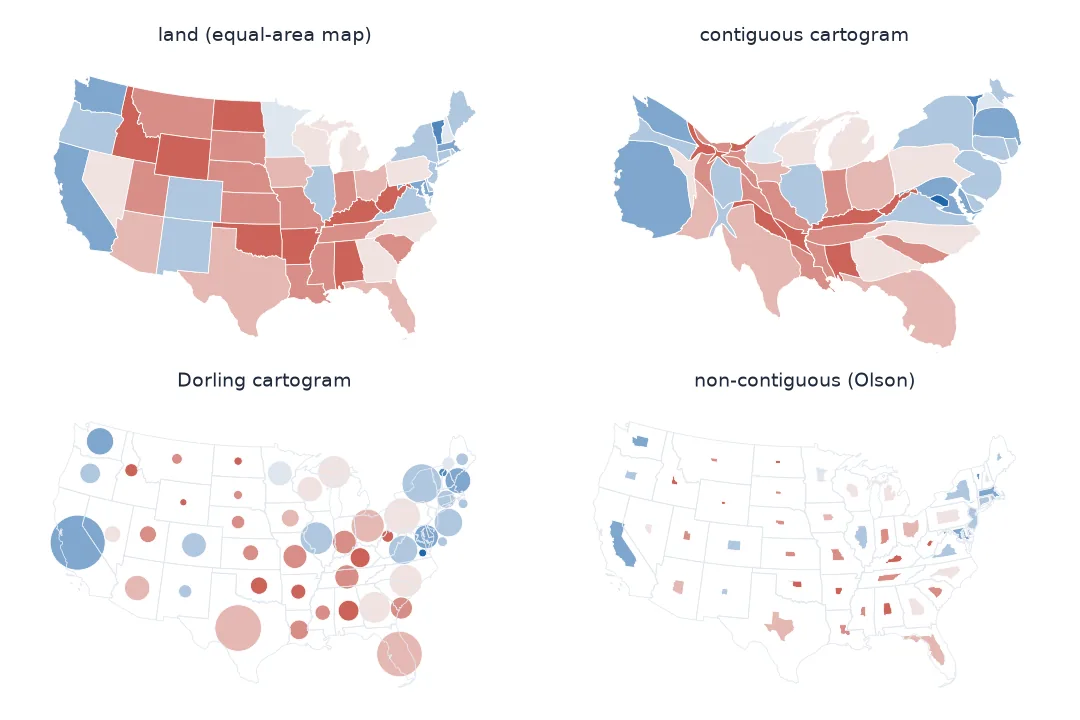
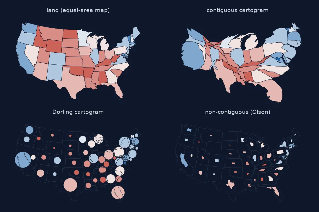
Four maps of the 2024 presidential margin by state. The equal-area map is dominated by large western states. The contiguous cartogram keeps borders but swells California, Texas, Florida and the Northeast and squeezes the mountain states. The Dorling cartogram replaces states with circles sized by votes near their real positions. The Olson cartogram shrinks each state in place inside its faint outline. — The same 2024 vote by state four ways. Data: county results compiled by tonmcg, summed to states; US Census Bureau boundaries.

An equal-area start, then contiguous, Dorling and non-contiguous

1. Start from an equal-area map

All cartograms are measured against an equal-area projection, because that is the map whose areas mean land. On it, more than a third of the map is in the "wrong" place for a vote map:

land = states.area / states.area.sum()
print(f"share of the map that would have to move to match votes: {np.abs(land - VOTE_SHARE).sum() / 2:.0%}")
print("most over-represented:", (land / VOTE_SHARE).nlargest(3).round(1).to_dict())
print("most under-represented:", (land / VOTE_SHARE).nsmallest(3).round(2).to_dict())

share of the map that would have to move to match votes: 38%
most over-represented: {'WY': 18.7, 'MT': 12.4, 'ND': 9.9}
most under-represented: {'DC': 0.01, 'NJ': 0.09, 'RI': 0.12}

2. Contiguous: keep the neighbours, bend the shapes

Contiguous cartograms move the boundaries themselves. Every region still touches the same neighbours, so the map can still be read as a map. The cost is shape: states with very high or very low density twist. This page uses the algorithm of Dougenik, Chrisman and Niemeyer (1985), 12 passes.

3. Dorling: keep size exactly, give up shape

Dorling cartograms replace each region with a circle of the right area and push overlapping circles apart. Area is exact, position is approximately right, and nothing of the shape survives. For thousands of small units, where a contiguous cartogram would tear itself apart, it is often the most readable choice.

4. Non-contiguous: keep shape and place, give up borders

Olson's method shrinks each region in place about its own centre. Shapes and positions are perfect, borders are lost, and the white space between regions shows how much each has shrunk. It needs an anchor region kept at full size, and an extreme outlier such as DC has to be capped.

What each method keeps and gives up.

Where each method puts California

The data used on this page

2024 presidential results by county from tonmcg/US_County_Level_Election_Results_08-24, summed to states; state boundaries from the US Census Bureau cartographic boundary files, 2023, 1:20 million, in EPSG:5070. Lower 48 states and DC.

from pathlib import Path

import geopandas as gpd
import numpy as np
import pandas as pd
import requests
import shapely
from scipy.spatial import cKDTree
from shapely import affinity

Path("data").mkdir(exist_ok=True)
for name, url in {"2024_US_County_Level_Presidential_Results.csv": "https://raw.githubusercontent.com/tonmcg/US_County_Level_Election_Results_08-24/master/2024_US_County_Level_Presidential_Results.csv",
                  "cb_2023_us_state_20m.zip": "https://www2.census.gov/geo/tiger/GENZ2023/shp/cb_2023_us_state_20m.zip"}.items():
    if not Path("data", name).exists():
        Path("data", name).write_bytes(requests.get(url, timeout=300).content)
res = pd.read_csv("data/2024_US_County_Level_Presidential_Results.csv", dtype={"county_fips": str})
states = gpd.read_file("data/cb_2023_us_state_20m.zip").query("STUSPS not in ['AK', 'HI', 'PR']").to_crs(5070)
states = states.join(res.groupby(res.county_fips.str[:2]).total_votes.sum(), on="STATEFP").set_index("STUSPS")
VOTE_SHARE = states.total_votes / states.total_votes.sum()


def dcn(geoms, values, passes=12):
    geoms = np.array(geoms, dtype=object)
    for _ in range(passes):
        area = shapely.area(geoms); desired = values / values.sum() * area.sum()
        c = shapely.get_coordinates(shapely.centroid(geoms)); radius = np.sqrt(area / np.pi)
        mass = np.sqrt(desired / np.pi) - radius
        reduce = 1 / (1 + (np.maximum(area, desired) / np.minimum(area, desired)).mean())
        xy = shapely.get_coordinates(geoms); shift = np.zeros_like(xy)
        for k in range(len(geoms)):
            d = xy - c[k]; dist = np.maximum(np.hypot(d[:, 0], d[:, 1]), 1e-9)
            f = np.where(dist > radius[k], mass[k] * radius[k] / dist, mass[k] * (dist / radius[k]) ** 2 * (4 - 3 * dist / radius[k]))
            shift += d / dist[:, None] * (f * reduce)[:, None]
        geoms = shapely.set_coordinates(geoms.copy(), xy + shift)
    return list(geoms)


def dorling(values, fill=0.35):
    pts = states.geometry.representative_point(); p = np.c_[pts.x, pts.y]
    r = np.sqrt(values / values.sum() * states.area.sum() * fill / np.pi)
    for _ in range(1000):
        pairs = cKDTree(p).query_pairs(2 * r.max(), output_type="ndarray")
        d = np.hypot(*(p[pairs[:, 0]] - p[pairs[:, 1]]).T); over = r[pairs[:, 0]] + r[pairs[:, 1]] - d
        hit = over > 1.0
        if not hit.any():
            break
        a, b = pairs[hit].T; u = (p[a] - p[b]) / np.maximum(d[hit], 1e-6)[:, None]
        w = r[b] ** 2 / (r[a] ** 2 + r[b] ** 2); move = np.zeros_like(p)
        np.add.at(move, a, u * (over[hit] * w)[:, None]); np.add.at(move, b, -u * (over[hit] * (1 - w))[:, None])
        p += move
    return [shapely.Point(x, y).buffer(rr, 64) for (x, y), rr in zip(p, r)]


def olson(values, anchor="NJ"):
    dens = values / states.area
    f = np.minimum(np.sqrt(dens / dens[anchor]), 1.0)
    return [affinity.scale(g, xfact=x, yfact=x, origin=g.centroid) for g, x in zip(states.geometry, f)]


def touching(geoms, tol=1_000):
    geoms = [g.buffer(tol / 2) for g in geoms]
    a, b = shapely.STRtree(geoms).query(geoms, predicate="intersects")
    return {(states.index[i], states.index[j]) for i, j in zip(a, b) if i < j}


def compactness(geoms):
    g = np.array(geoms, dtype=object)
    return 4 * np.pi * shapely.area(g) / shapely.length(g) ** 2


REAL = touching(list(states.geometry))
BASE_SHAPE = compactness(list(states.geometry))
v = states.total_votes.values.astype(float)
METHODS = {"equal-area map": list(states.geometry), "contiguous": dcn(states.geometry.values, v),
           "Dorling": dorling(v), "Olson": olson(states.total_votes)}
print(f"{len(states)} regions; {len(REAL)} pairs of states that touch")

49 regions; 109 pairs of states that touch

Example 1: where each method puts California

for name, geoms in METHODS.items():
    a = shapely.area(np.array(geoms, dtype=object))
    i = list(states.index).index("CA")
    print(f"{name:15s}: California {a[i] / a.sum():.1%} of the map (votes {VOTE_SHARE['CA']:.1%}, land {states.area['CA'] / states.area.sum():.1%})")

equal-area map : California 5.2% of the map (votes 10.3%, land 5.2%)
contiguous     : California 10.2% of the map (votes 10.3%, land 5.2%)
Dorling        : California 10.3% of the map (votes 10.3%, land 5.2%)
Olson          : California 10.3% of the map (votes 10.3%, land 5.2%)

Where California ends up.

A map that changes its measure of area

A cartogram is a map that changes its measure of area. Once area means votes or people instead of land, the map can no longer keep every other property, because the shapes of real regions do not tile the plane in proportion to population. Something must give. Contiguous cartograms give up shape. Dorling cartograms give up shape and borders and keep only size and rough position. Non-contiguous cartograms give up borders and keep shape and position, at the cost of empty space and an arbitrary anchor.

Choosing a cartogram; always pair it with a normal map.

The right choice depends on what readers need to do. If they must find their region by its outline and see who borders whom, use a contiguous cartogram, and keep the ratio of values moderate. If they need exact comparisons across thousands of units, use Dorling circles. If they need to see how much each region shrinks relative to its land, use Olson. Pair any of them with a normal map: cartograms are read by comparison with the geography readers already know.

Extreme ratios, tile maps and legends

Common cartogram mistakes. Wyoming has 18.7 times its vote share in land.

Start from an equal-area projection; cartograms from Web Mercator inherit its distortions.
Extreme ratios break contiguous cartograms; switch to Dorling or Olson, or soften the target and say so.
Tile and hex maps are cartograms where every unit gets the same area.
Value-by-alpha is an alternative that keeps the geography and fades sparse areas instead of shrinking them.
Legends should state the variable that sets area and, for Olson, the anchor.
Cartogram coordinates are not geography; never measure distance or overlay data on them.

Internal links

FAQ

What is a cartogram?

A map in which each region's area is proportional to a chosen value, such as population or votes, rather than to its land area.

What are the main types of cartogram?

Contiguous (boundaries bend, neighbours kept), Dorling (circles sized by value), non-contiguous or Olson (regions shrink in place), and tile or hex maps (equal shapes for equal units).

Which cartogram is most accurate?

Dorling and Olson make area exactly proportional; contiguous cartograms approach it iteratively and trade some accuracy for shape.

Why use a cartogram instead of a normal map?

Because on a normal map large, sparsely populated regions dominate; a cartogram gives visual weight in proportion to the thing being mapped.