How to Make a Dot-Density Election Map in Python

Problem statement

A dot-density map draws one dot for every so many votes, in the party's colour, inside the area where they were cast. It solves the two problems of a choropleth at once. Empty land stays empty, because there are no votes to draw there. And a close race looks mixed, because red and blue dots sit side by side instead of one colour winning the whole county. Making one well takes four decisions: how many votes a dot stands for, how to round, where inside each area to put the dots, and in what order to draw them.

This page builds a dot-density map of the 2024 presidential vote in Arizona, a close state with one huge county. It uses the county results and the GHSL population grid to place the dots, and measures the effect of each decision.

Quick answer

For each county and party, draw one dot per 1,000 votes, placed at random among the 1 km population cells of the county in proportion to how many people live there, then shuffle all dots before plotting:

def place(geom, n, rng):
    arr, tr = mask(pop, [geom], crop=True, nodata=0)
    weight = np.maximum(arr[0], 0).ravel()
    cells = rng.choice(weight.size, n, p=weight / weight.sum())
    row, col = np.unravel_index(cells, arr[0].shape)
    return np.c_[tr.c + (col + rng.random(n)) * tr.a, tr.f + (row + rng.random(n)) * tr.e]   # jitter inside the cell

rng = np.random.default_rng(42)
dots = []
for _, cty in az.iterrows():
    for party, colour in (("gop", "#c0392b"), ("dem", "#2166ac")):
        n = stochastic_round(cty[f"votes_{party}"] / VOTES_PER_DOT, rng)
        dots.append(pd.DataFrame(place(cty.geometry, n, rng), columns=["x", "y"]).assign(colour=colour))
dots = pd.concat(dots).sample(frac=1, random_state=1)                    # shuffle: no party drawn on top
print(f"{len(dots):,} dots for {az[['votes_gop', 'votes_dem']].sum().sum():,} two-party votes")

3,355 dots for 3,353,102 two-party votes

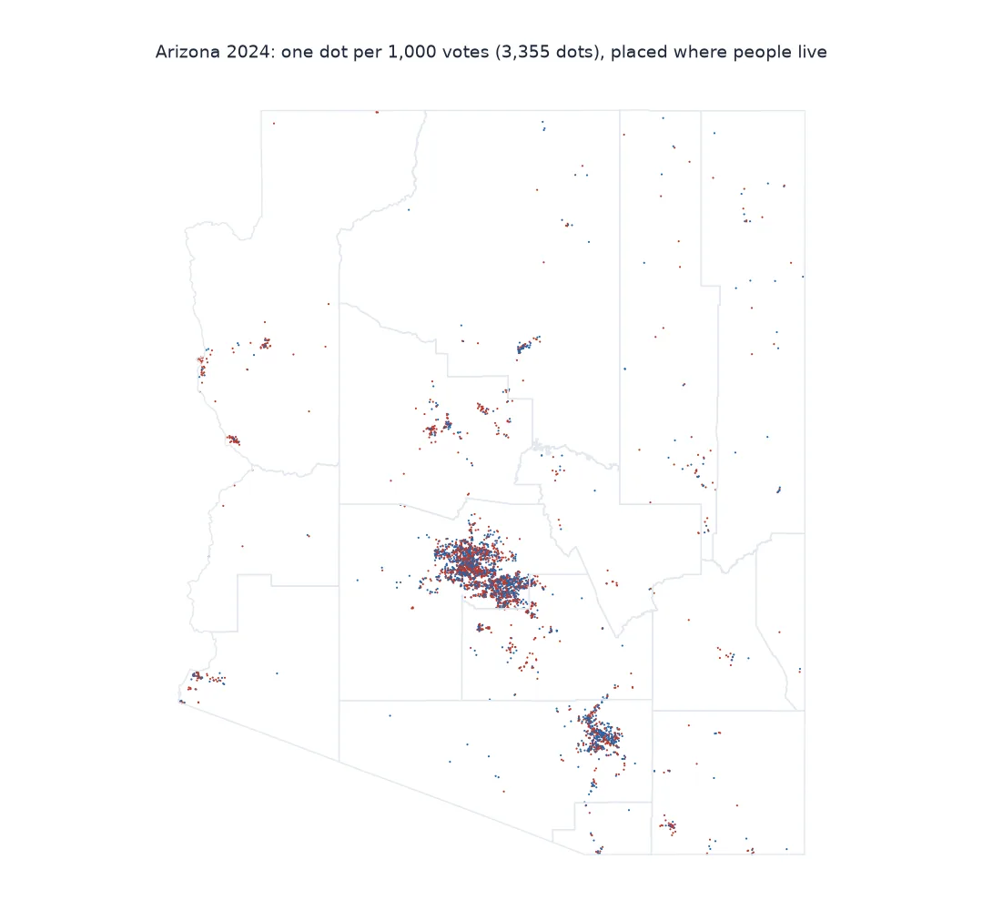
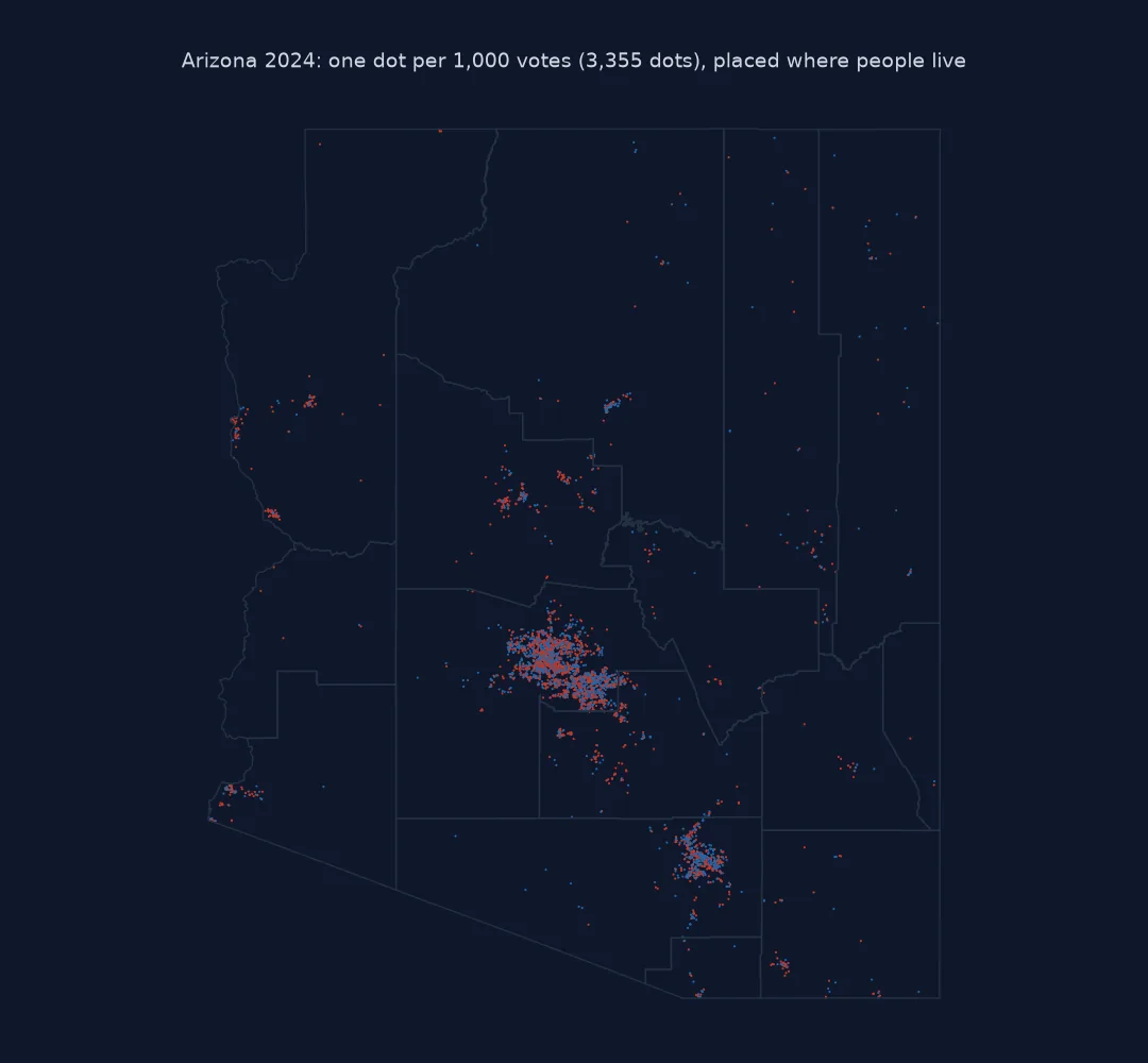
Dot value, unbiased rounding, dots where people live

1. Choose the dot value

The dot value trades detail against clutter. Too few votes per dot and the cities become solid blobs; too many and small towns vanish:

for per_dot in (100, 1_000, 10_000):
    n = (az.votes_gop / per_dot).round() + (az.votes_dem / per_dot).round()
    print(f"1 dot = {per_dot:>6,} votes: {int(n.sum()):>6,} dots; {(n == 0).sum()} of {len(az)} counties get no dot; "
          f"Maricopa alone {int(n[az.NAME == 'Maricopa'].iloc[0]):,}")

1 dot =    100 votes: 33,532 dots; 0 of 15 counties get no dot; Maricopa alone 20,315
1 dot =  1,000 votes:  3,355 dots; 0 of 15 counties get no dot; Maricopa alone 2,032
1 dot = 10,000 votes:    335 dots; 1 of 15 counties get no dot; Maricopa alone 203

Maricopa County casts about 60% of Arizona's votes. At one dot per 1,000 votes the smallest county still gets a handful of dots, and Phoenix stays readable at a state-wide scale.

2. Round without bias

Plain rounding per county and party loses or invents votes, and at coarse dot values it erases the minority party in small counties. Stochastic rounding keeps the fractional part as a probability, so the expected count is exact:

for per_dot in (1_000, 10_000):
    exact = az.votes_dem.sum() / per_dot
    plain = sum(round(v / per_dot) for v in az.votes_dem)
    draws = [sum(stochastic_round(v / per_dot, np.random.default_rng(s)) for v in az.votes_dem) for s in range(200)]
    erased = az[(az.votes_dem / per_dot).round() == 0].NAME.tolist()
    print(f"1 dot = {per_dot:,}: exact {exact:.1f}, plain {plain}, stochastic mean {np.mean(draws):.1f}; "
          f"counties whose Democratic votes plain rounding erases: {erased}")

1 dot = 1,000: exact 1582.9, plain 1584, stochastic mean 1582.2; counties whose Democratic votes plain rounding erases: []
1 dot = 10,000: exact 158.3, plain 157, stochastic mean 157.8; counties whose Democratic votes plain rounding erases: ['Graham', 'La Paz', 'Greenlee']

At 1,000 votes per dot plain rounding is almost harmless in Arizona. At 10,000 it starts deleting whole counties' minority vote, while stochastic rounding still gives them a dot in proportion to their votes, on average.

3. Put the dots where people live

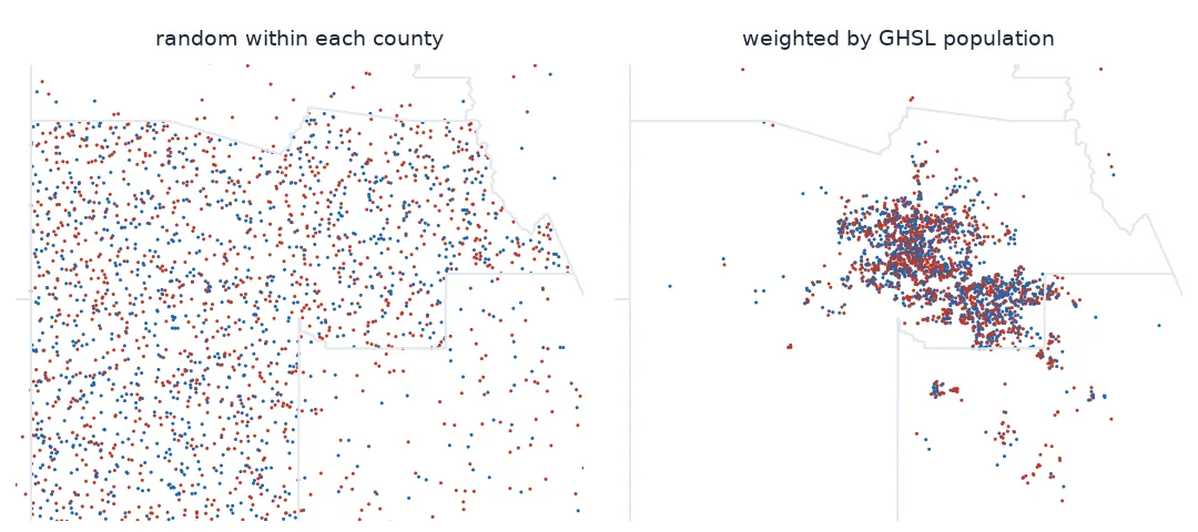
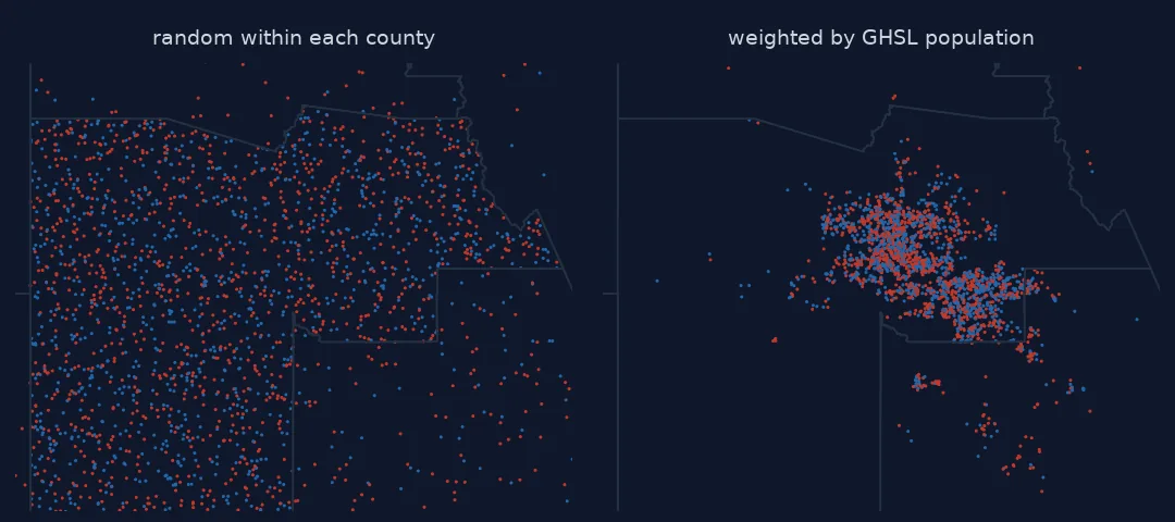
The simplest placement scatters dots uniformly within each county. In a state of deserts, mountains and reservations that puts most dots where almost nobody lives. Weighting by a population grid keeps them in towns and cities:

def uniform(geom, n, rng):
    pts = np.empty((0, 2)); x0, y0, x1, y1 = geom.bounds
    while len(pts) < n:
        x, y = rng.uniform(x0, x1, 3 * n + 10), rng.uniform(y0, y1, 3 * n + 10)
        pts = np.vstack([pts, np.c_[x, y][shapely.contains_xy(geom, x, y)]])
    return pts[:n]

u = np.vstack([uniform(cty.geometry, int(round(cty.total_votes / VOTES_PER_DOT)), rng) for _, cty in az.iterrows()])
people_u = np.array([v[0] for v in pop.sample(map(tuple, u))])
people_w = np.array([v[0] for v in pop.sample(map(tuple, dots[["x", "y"]].to_numpy()))])
print(f"dots in 1 km cells with under 1 resident: uniform {np.mean(people_u < 1):.0%}, population-weighted {np.mean(people_w < 1):.1%}")

dots in 1 km cells with under 1 resident: uniform 83%, population-weighted 0.1%

4. Draw in a shuffled order

fig, ax = plt.subplots(figsize=(7, 8))
ax.scatter(dots.x, dots.y, s=1, c=dots.colour, linewidths=0)
ax.set_aspect(1 / np.cos(np.radians(34))); ax.set_axis_off()
fig.savefig("data/arizona_dots.png", dpi=200)
first_gop = (dots.colour.iloc[: len(dots) // 2] == "#c0392b").mean()
print(f"Republican share of the first half drawn: {first_gop:.1%} (shuffled; unshuffled it would be 100% or 0%)")

Republican share of the first half drawn: 52.8% (shuffled; unshuffled it would be 100% or 0%)

If all of one party's dots are drawn first, the other party's dots sit on top of them in every city, and the map's colour depends on drawing order rather than votes.

What the dots say about Maricopa

The data used on this page

2024 presidential results by county from tonmcg/US_County_Level_Election_Results_08-24; Arizona counties from the US Census Bureau cartographic boundary files, 2023, 1:500,000; population from the European Commission JRC GHS-POP R2023A grid for 2020 at 30 arc-seconds (about 1 km), tiles R6_C7 and R6_C8.

import zipfile
from pathlib import Path

import geopandas as gpd
import matplotlib
matplotlib.use("Agg")
import matplotlib.pyplot as plt
import numpy as np
import pandas as pd
import rasterio
import requests
import shapely
from rasterio.mask import mask
from rasterio.merge import merge

Path("data").mkdir(exist_ok=True)
GHS = ("https://jeodpp.jrc.ec.europa.eu/ftp/jrc-opendata/GHSL/GHS_POP_GLOBE_R2023A/GHS_POP_E2020_GLOBE_R2023A_4326_30ss/V1-0/tiles/"
       "GHS_POP_E2020_GLOBE_R2023A_4326_30ss_V1_0_R6_C{}.zip")
SOURCES = {"2024_US_County_Level_Presidential_Results.csv": "https://raw.githubusercontent.com/tonmcg/US_County_Level_Election_Results_08-24/master/2024_US_County_Level_Presidential_Results.csv",
           "cb_2023_us_county_500k.zip": "https://www2.census.gov/geo/tiger/GENZ2023/shp/cb_2023_us_county_500k.zip",
           "ghs_R6_C7.zip": GHS.format(7), "ghs_R6_C8.zip": GHS.format(8)}
for name, url in SOURCES.items():
    if not Path("data", name).exists():
        Path("data", name).write_bytes(requests.get(url, timeout=600).content)
tiles = []
for c in (7, 8):
    tif = f"GHS_POP_E2020_GLOBE_R2023A_4326_30ss_V1_0_R6_C{c}.tif"
    if not Path("data", tif).exists():
        zipfile.ZipFile(f"data/ghs_R6_C{c}.zip").extract(tif, "data")
    tiles.append(rasterio.open(Path("data", tif)))
arr, tr = merge(tiles, bounds=(-115.0, 31.2, -108.9, 37.1))
profile = tiles[0].profile | {"height": arr.shape[1], "width": arr.shape[2], "transform": tr}
with rasterio.open("data/ghs_pop_arizona.tif", "w", **profile) as dst:
    dst.write(arr)
pop = rasterio.open("data/ghs_pop_arizona.tif")

res = pd.read_csv("data/2024_US_County_Level_Presidential_Results.csv", dtype={"county_fips": str}).set_index("county_fips")
az = gpd.read_file("data/cb_2023_us_county_500k.zip").query("STATEFP == '04'").to_crs(4326)
az = az.join(res[["votes_gop", "votes_dem", "total_votes"]], on="GEOID")
VOTES_PER_DOT = 1_000


def stochastic_round(x, rng):
    """Round down, then up with probability equal to the fraction: unbiased on average."""
    return int(np.floor(x) + (rng.random() < x - np.floor(x)))


print(f"{len(az)} counties, {az.total_votes.sum():,} votes; GHSL grid {pop.width} x {pop.height} cells")

15 counties, 3,389,319 votes; GHSL grid 732 x 708 cells

Example 1: what the dots say about Maricopa

m = dots.assign(maricopa=[az[az.NAME == "Maricopa"].geometry.iloc[0].contains(shapely.Point(x, y)) for x, y in zip(dots.x, dots.y)])
share = m.groupby("maricopa").colour.apply(lambda c: (c == "#c0392b").mean())
print(f"Maricopa holds {m.maricopa.mean():.0%} of the dots; Republican share of dots inside {share[True]:.1%}, outside {share[False]:.1%}")

Maricopa holds 61% of the dots; Republican share of dots inside 51.7%, outside 54.4%

Example 2: export the dots

gpd.GeoDataFrame(dots, geometry=gpd.points_from_xy(dots.x, dots.y), crs=4326).to_file("data/arizona_dots.gpkg")
print(Path("data/arizona_dots.gpkg").stat().st_size // 1000, "kB; each point is a random draw, not a voter's location")

495 kB; each point is a random draw, not a voter's location

Quantity as marks, composition as colour

A dot-density map encodes quantity as the number of marks and composition as their colours. Unlike a choropleth, it does not average a county into one colour. Unlike proportional symbols, it does not need a legend for size. The eye reads density and mix directly. The dots are not locations: each is a random draw constrained to the right county and, ideally, to inhabited land. The map must say so, and it must never be zoomed to street level, where the randomness becomes visible as fake precision.

The decisions compound. The dot value sets what is visible. Rounding decides whether small places and minority votes appear at all. Placement decides whether the map shows people or land. Draw order decides which colour wins where dots overlap. Get all four right and the result is one of the most honest pictures of an election there is.

Residents against voters, dot size and colour vision

• Population is not turnout: GHSL counts residents in 2020, not voters in 2024; weighting by it moves dots towards where people live, not exactly where they voted.
• Dot size and map scale go together; resize dots when the output size changes.
• Colour-blind readers need a palette that works without red-green contrast; red-blue does.
• Very large counties with one town can concentrate all dots in a few cells; that is correct.
• Re-running with another seed moves every dot; fix the seed for reproducible maps.
• Precinct results, where available, give far better placement than county totals.

Internal links

• Dot-density dots in the wrong places — the placement problem in depth
• How to make a US county election map — the choropleth this replaces
• How to make a Dorling cartogram — another way to show votes, not land

FAQ

How do I make a dot density map in Python?

For each area and category, compute the number of dots (value ÷ dot value, rounded stochastically), place random points inside the area — ideally weighted by a population grid — shuffle all points, and plot them with scatter.

How many votes should one dot represent?

Enough that the densest area does not become a solid blob and small enough that the smallest area still gets a few dots; for Arizona, 1,000 votes per dot gives about 3,400 dots.

Why are my dots in empty desert?

Uniform random placement ignores where people live; weight placement by a population grid such as GHSL.

Should dots be drawn in a particular order?

Shuffle them. Drawing one party first lets the other cover it wherever dots overlap.