How to Make a Non-Contiguous Cartogram in Python

On this page

Problem statement

A non-contiguous cartogram shrinks every region in place, about its own centre, until its area is proportional to a value. Shapes stay exactly as they are, so every state is recognisable, and the gaps that open between them show how much smaller each region is than its share of the land. Judith Olson described the method in 1976. It is the easiest cartogram to compute, a single scale factor per region, and the easiest to read.

The method hides one real decision: which region stays full size. Every other region is scaled relative to that anchor. This page builds the cartogram of the 2024 presidential vote by state. It shows how the anchor choice decides whether the map is readable, and measures the overlaps that can appear even though every region only shrinks or holds its size.

Quick answer

Scale each region about its centroid by the square root of its value density relative to the anchor's, capping the scale at 1:

density = states.total_votes / states.area
anchor = density[states.STUSPS == "NJ"].iloc[0]                     # the densest real state, not DC
factor = np.minimum(np.sqrt(density / anchor), 1.0)                 # area scales with factor squared
shrunk = [affinity.scale(g, xfact=f, yfact=f, origin=g.centroid) for g, f in zip(states.geometry, factor)]
print(f"map keeps {shapely.area(np.array(shrunk)).sum() / states.area.sum():.1%} of the land area; "
      f"factors {factor.min():.3f}–{factor.max():.2f}")

map keeps 9.3% of the land area; factors 0.070–1.00

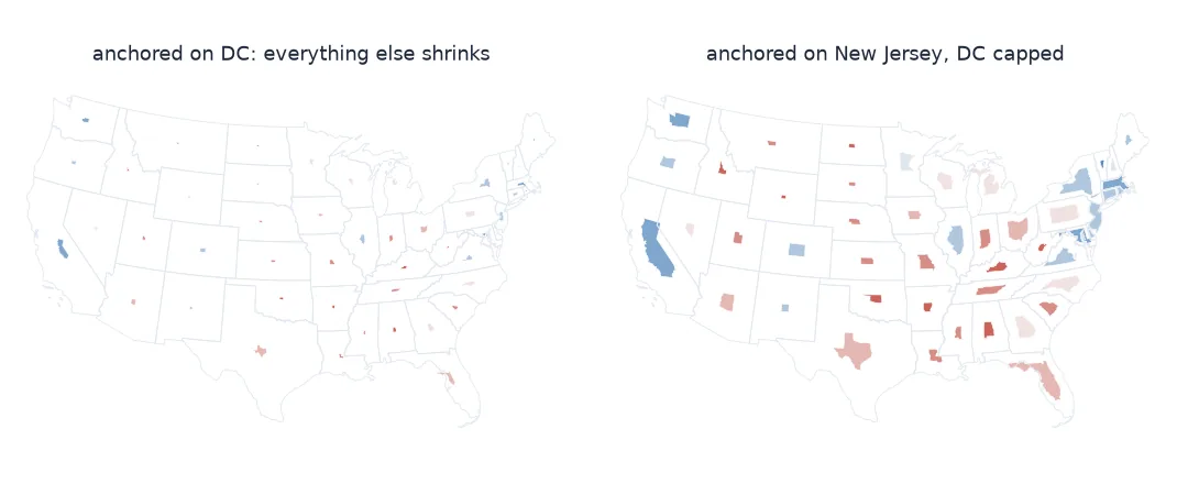
Two non-contiguous cartograms of the 2024 presidential margin over faint real state outlines. Anchored on DC, every state shrinks to a small speck, with California and Florida barely visible. Anchored on New Jersey with DC capped, the eastern states keep much of their size, California, New York and Florida are clearly visible, and the western and plains states shrink to small shapes in the middle of their outlines. — Two anchors for the same cartogram. Data: county results compiled by tonmcg, summed to states; US Census Bureau boundaries.

Scale factors, anchors, overlaps, real outlines behind

1. Work out the scale factors

If a region's area should be proportional to its value, its area must be multiplied by the ratio of its density (value per area) to the anchor's. Linear dimensions scale by the square root of that:

f_all = np.sqrt(density / density.max())
show = states.assign(factor=f_all, votes_per_km2=density * 1e6)[["STUSPS", "votes_per_km2", "factor"]]
print(show.sort_values("factor").iloc[[0, 1, 2, -3, -2, -1]].round(3).to_string(index=False))

STUSPS  votes_per_km2  factor
    WY          1.051   0.024
    MT          1.584   0.029
    ND          1.993   0.033
    RI        159.388   0.296
    NJ        211.683   0.341
    DC       1821.155   1.000

2. Choose the anchor

The obvious anchor is the densest region. Here that is the District of Columbia, a city, with several times the vote density of any state. Anchor on it and everything else becomes a speck:

for code, cap in ((None, 1.0), ("NJ", 1.0)):
    ref = density.max() if code is None else density[states.STUSPS == code].iloc[0]
    f = np.minimum(np.sqrt(density / ref), cap)
    kept = (states.area * f ** 2).sum() / states.area.sum()
    print(f"anchor {code or 'DC (densest)'}: map keeps {kept:.1%} of the land area; California factor {f[states.STUSPS == 'CA'].iloc[0]:.2f}")

anchor DC (densest): map keeps 1.1% of the land area; California factor 0.15
anchor NJ: map keeps 9.3% of the land area; California factor 0.43

Anchoring on the densest state, New Jersey, and capping DC at its real size keeps a readable map. DC is then smaller than its share, which a note on the map should say. The choice is a design decision, not a technical one. Make it on purpose and report it.

The anchor sets the scale for the whole map.

3. Check for overlaps

Shrinking a shape about its centroid moves every part of it towards that point. For a concave state the shrunken outline can still cross into a neighbour that stayed large:

tree = shapely.STRtree(shrunk)
a, b = tree.query(shrunk, predicate="intersects")
hits = [(states.STUSPS[i], states.STUSPS[j], shapely.intersection(shrunk[i], shrunk[j]).area / 1e6)
        for i, j in zip(a, b) if i < j and shapely.intersection(shrunk[i], shrunk[j]).area > 0]
print([(x, y, round(km2, 1)) for x, y, km2 in hits])

[('MD', 'DC', 4.9), ('MA', 'RI', 28.2), ('DE', 'NJ', 51.7)]

The overlaps are small, at most tens of square kilometres, and each involves a region kept at full or nearly full size. Shrinking everything a little more does not clear them all:

for k in (0.95, 0.9, 0.8, 0.7):
    g = [affinity.scale(s, xfact=f * k, yfact=f * k, origin=s.centroid) for s, f in zip(states.geometry, factor)]
    a, b = shapely.STRtree(g).query(g, predicate="intersects")
    left = [(states.STUSPS[i], states.STUSPS[j]) for i, j in zip(a, b) if i < j and shapely.intersection(g[i], g[j]).area > 0]
    print(f"all factors x {k}: {left}")

all factors x 0.95: [('MD', 'DC'), ('MA', 'RI'), ('DE', 'NJ')]
all factors x 0.9: [('MA', 'RI')]
all factors x 0.8: [('MA', 'RI')]
all factors x 0.7: []

Massachusetts wraps around Rhode Island on two sides, so shrinking both about their centroids keeps pushing them into each other until the whole map is 30% smaller. Fix the pairs instead: shrink only the regions that overlap, a step at a time:

fixed = factor.copy()
for _ in range(50):
    g = [affinity.scale(s, xfact=f, yfact=f, origin=s.centroid) for s, f in zip(states.geometry, fixed)]
    a, b = shapely.STRtree(g).query(g, predicate="intersects")
    pairs = [(i, j) for i, j in zip(a, b) if i < j and shapely.intersection(g[i], g[j]).area > 0]
    if not pairs:
        break
    for i, j in pairs:
        fixed.iloc[[i, j]] *= 0.97
changed = states.STUSPS[fixed < factor].tolist()
print(f"no overlaps after {_} rounds; adjusted {changed}, by up to {(1 - (fixed / factor).min()):.0%}")
shrunk = g

no overlaps after 8 rounds; adjusted ['MD', 'DC', 'MA', 'RI', 'DE', 'NJ'], by up to 22%

4. Draw it over the real outlines

The faint real outlines give the eye the scale the shrunken shapes are measured against:

fig, ax = plt.subplots(figsize=(10, 6))
states.boundary.plot(ax=ax, color="#d0d0d0", linewidth=0.4)
gpd.GeoDataFrame(states[["margin"]], geometry=shrunk, crs=states.crs).plot(ax=ax, column="margin", cmap="RdBu_r", vmin=-0.6, vmax=0.6)
ax.set_axis_off(); fig.savefig("data/olson_2024.png", dpi=150)
print("saved")

saved

How much each state shrinks

The data used on this page

2024 presidential results by county from tonmcg/US_County_Level_Election_Results_08-24, summed to states; state boundaries from the US Census Bureau cartographic boundary files, 2023, 1:20 million.

from pathlib import Path

import geopandas as gpd
import matplotlib
matplotlib.use("Agg")
import matplotlib.pyplot as plt
import numpy as np
import pandas as pd
import requests
import shapely
from shapely import affinity

Path("data").mkdir(exist_ok=True)
for name, url in {"2024_US_County_Level_Presidential_Results.csv": "https://raw.githubusercontent.com/tonmcg/US_County_Level_Election_Results_08-24/master/2024_US_County_Level_Presidential_Results.csv",
                  "cb_2023_us_state_20m.zip": "https://www2.census.gov/geo/tiger/GENZ2023/shp/cb_2023_us_state_20m.zip"}.items():
    if not Path("data", name).exists():
        Path("data", name).write_bytes(requests.get(url, timeout=300).content)
res = pd.read_csv("data/2024_US_County_Level_Presidential_Results.csv", dtype={"county_fips": str})
states = gpd.read_file("data/cb_2023_us_state_20m.zip").query("STUSPS not in ['AK', 'HI', 'PR']").to_crs(5070).reset_index(drop=True)
states = states.join(res.groupby(res.county_fips.str[:2])[["votes_gop", "votes_dem", "total_votes"]].sum(), on="STATEFP")
states["margin"] = (states.votes_gop - states.votes_dem) / states.total_votes
print(f"{len(states)} regions in EPSG:5070")

49 regions in EPSG:5070

Example 1: how much each state shrinks

shr = states.assign(area_left=factor ** 2)[["STUSPS", "area_left"]].sort_values("area_left")
print("smallest:", shr.head(4).round(4).values.tolist())
print("largest :", shr.tail(4).round(3).values.tolist())
red = states.margin > 0
a = shapely.area(np.array(shrunk))
print(f"Republican-won share of the cartogram's area {a[red].sum() / a.sum():.0%}, of the land {states.area[red].sum() / states.area.sum():.0%}")

smallest: [['WY', 0.005], ['MT', 0.0075], ['ND', 0.0094], ['SD', 0.0101]]
largest : [['MA', 0.744], ['RI', 0.753], ['DC', 1.0], ['NJ', 1.0]]
Republican-won share of the cartogram's area 60%, of the land 71%

What each kind of cartogram keeps and gives up.

Shape and position kept, contiguity given up

Contiguous cartograms keep the neighbours and give up the shapes; Dorling cartograms give up both and keep only size and rough position. Olson's non-contiguous cartogram keeps shape and position and gives up contiguity. The white space between regions is part of the message: a state that has shrunk to a tenth of its outline tells you at once how thinly its land is populated relative to the anchor.

Building an Olson cartogram. A global factor had to fall to 0.7 to separate Massachusetts and Rhode Island.

Its weakness is the anchor. The whole map is scaled to one region, so an outlier, such as a city-district like DC or a microstate in a map of Europe, can shrink everything else to illegibility. Anchoring on a typical dense region and capping the outliers keeps the map readable at the cost of making those few regions too small, a trade worth stating on the map.

Area against linear size, multipart regions and overlaps

Olson cartogram problems and fixes.

Area, not linear size, must be proportional: use the square root of the density ratio as the linear factor.
Multipart regions (Michigan, islands) scale about the whole region's centroid, so the parts move closer together.
Very small factors turn states into dots; add labels or a minimum size and say so.
Overlaps can appear next to full-size regions; shrink only the overlapping pairs rather than the whole map.
The anchor must be stated; it sets the scale for everything.
Equal-area projection first: scale factors computed in a non-equal-area CRS are meaningless.

Internal links

How to make a contiguous cartogram — keeping neighbours
How to make a Dorling cartogram — circles instead of shapes
Choosing a projected CRS — start from equal area

FAQ

What is a non-contiguous cartogram?

A cartogram in which each region is scaled about its own centre so its area is proportional to a value; regions keep their shapes but no longer touch.

How do I compute the scale factor for each region?

The square root of the region's value density divided by the anchor's density, so that the region's area scales by the density ratio.

Which region should stay full size?

Usually the densest typical region; a single extreme outlier, such as a city district, shrinks everything else to illegibility and is better capped.

Why do some regions overlap in my non-contiguous cartogram?

Shrinking a shape about its centroid can push part of it into a neighbour that stayed large or wraps around it; shrink just the overlapping pair a few percent at a time until they separate.