Cartogram Distorted Beyond Recognition: Twisted Shapes and Invalid Polygons

Problem statement

You run a contiguous cartogram on small units — counties, districts, municipalities — and the result is unreadable. Shapes stretch into spikes and thin necks, rural areas collapse into slivers threading between swollen cities, and some polygons become invalid, crossing over themselves so that GeoPandas refuses to clip or dissolve them. The algorithm is doing what it was asked. The ratio between the largest and smallest values is so extreme that no contiguous map can satisfy it without tearing the shapes apart.

This page reproduces the failure with the 2024 presidential vote across Texas's 254 counties, where the largest county cast 16,000 times as many votes as the smallest. It measures the damage pass by pass and compares the fixes: fewer passes, denser outlines, a softened target, repaired geometry, and switching to a Dorling cartogram.

Quick answer

Measure the value ratio before you start, monitor validity and shape as well as size error, and change the target or the method when the ratio is extreme:

print(f"{len(tx)} counties; largest/smallest votes ratio {tx.total_votes.max() / tx.total_votes.min():,.0f}")
g = tx.geometry.values
for p in range(1, 31):
    g = cartogram_pass(g, tx.total_votes.values.astype(float))
    if p in (5, 10, 20, 30):
        print(f"pass {p:2d}: mean size error {size_error(g, tx.total_votes.values):5.2f}, invalid {(~shapely.is_valid(g)).sum():2d}, "
              f"median compactness {np.median(compactness(g)) / BASE:.2f} of the original")

254 counties; largest/smallest votes ratio 16,044
pass  5: mean size error 15.57, invalid  0, median compactness 0.90 of the original
pass 10: mean size error 10.22, invalid  1, median compactness 0.72 of the original
pass 20: mean size error  2.38, invalid 21, median compactness 0.28 of the original
pass 30: mean size error  1.50, invalid 65, median compactness 0.18 of the original

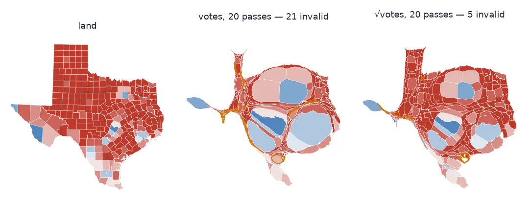
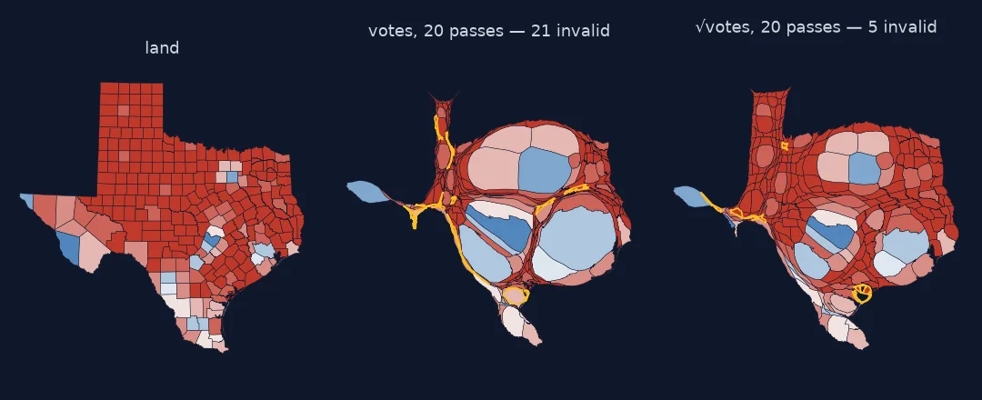
The ratio, stopping earlier, denser outlines, softer targets

1. Recognise the cause: the ratio

A contiguous cartogram must make every region's area proportional to its value while keeping its borders. When a few regions must grow enormously and their neighbours shrink to almost nothing, the shrinking ones have to become thin strips between the giants:

share_votes = tx.total_votes / tx.total_votes.sum()
share_land = tx.area / tx.area.sum()
growth = (share_votes / share_land).sort_values()
print(f"must shrink most: {growth.index[0]} x{growth.iloc[0]:.4f}; must grow most: {growth.index[-1]} x{growth.iloc[-1]:.0f}")
print(f"counties that must shrink below a tenth of their area: {(growth < 0.1).sum()} of {len(tx)}")

must shrink most: Kenedy x0.0024; must grow most: Dallas x22
counties that must shrink below a tenth of their area: 92 of 254

2. Stop earlier — up to a point

The size error falls fast at first; the damage accumulates later. Stopping at the pass where the error is good enough trades accuracy for readability, but in Texas the error is still large when shapes start to break.

3. Densify the outlines

Every vertex moves independently. Long straight segments between far-apart vertices cut corners when their ends move differently, which is how self-intersections start. Adding vertices helps:

dense = shapely.segmentize(tx.geometry.values, 2000)                    # a vertex at least every 2 km
g = dense
for p in range(20):
    g = cartogram_pass(g, tx.total_votes.values.astype(float))
print(f"densified, 20 passes: {len(shapely.get_coordinates(dense)):,} vertices, invalid {(~shapely.is_valid(g)).sum()}, "
      f"compactness {np.median(compactness(g)) / BASE:.2f}")

densified, 20 passes: 88,024 vertices, invalid 4, compactness 0.28

It reduces the number of broken polygons but does not remove the underlying distortion.

4. Soften the target, and say so

Sizing by the square root of the votes is a partial cartogram: big counties still grow and small ones still shrink, but less. It is no longer "area proportional to votes", and the map must say what it shows:

g_sqrt = tx.geometry.values
for p in range(20):
    g_sqrt = cartogram_pass(g_sqrt, np.sqrt(tx.total_votes.values))
a = shapely.area(g_sqrt)
harris = (tx.NAME == "Harris").to_numpy()
print(f"sqrt target, 20 passes: invalid {(~shapely.is_valid(g_sqrt)).sum()}, compactness {np.median(compactness(g_sqrt)) / BASE:.2f}")
print(f"Harris County: {share_land[harris].iloc[0]:.2%} of the land, {a[harris][0] / a.sum():.1%} of this map, {share_votes[harris].iloc[0]:.1%} of the votes")

sqrt target, 20 passes: invalid 5, compactness 0.64
Harris County: 0.67% of the land, 3.6% of this map, 13.7% of the votes

5. Repair what is left, or change method

Invalid polygons can be repaired, though the repair may split a twisted county into pieces:

fixed = shapely.make_valid(g_sqrt)
before = shapely.get_num_geometries(tx.geometry.values)
print(f"after make_valid: invalid {(~shapely.is_valid(fixed)).sum()}; counties in more than one piece: "
      f"{(shapely.get_num_geometries(fixed) > 1).sum()} (before the cartogram: {(before > 1).sum()})")

after make_valid: invalid 0; counties in more than one piece: 15 (before the cartogram: 11)

The repair works, but four counties come out in more pieces than they started with. For extreme ratios the honest alternative is to give up contiguity. A Dorling cartogram puts exact sizes on circles and needs no shape at all:

pts = tx.geometry.representative_point()
r = np.sqrt(tx.total_votes / tx.total_votes.sum() * tx.area.sum() * 0.12 / np.pi).values
moved, passes = dorling(np.c_[pts.x, pts.y], r)
shift = np.hypot(*(moved - np.c_[pts.x, pts.y]).T) / 1000
print(f"Dorling: no overlaps after {passes} passes; median move {np.median(shift):.1f} km, max {shift.max():.0f} km")

Dorling: no overlaps after 21 passes; median move 0.0 km, max 33 km

Which counties break first

The data used on this page

2024 presidential results by county from tonmcg/US_County_Level_Election_Results_08-24; Texas counties from the US Census Bureau cartographic boundary files, 2023, 1:500,000, in Texas Centric Albers Equal Area (EPSG:3083).

from pathlib import Path

import geopandas as gpd
import numpy as np
import pandas as pd
import requests
import shapely
from scipy.spatial import cKDTree

Path("data").mkdir(exist_ok=True)
for name, url in {"2024_US_County_Level_Presidential_Results.csv": "https://raw.githubusercontent.com/tonmcg/US_County_Level_Election_Results_08-24/master/2024_US_County_Level_Presidential_Results.csv",
                  "cb_2023_us_county_500k.zip": "https://www2.census.gov/geo/tiger/GENZ2023/shp/cb_2023_us_county_500k.zip"}.items():
    if not Path("data", name).exists():
        Path("data", name).write_bytes(requests.get(url, timeout=300).content)
res = pd.read_csv("data/2024_US_County_Level_Presidential_Results.csv", dtype={"county_fips": str}).set_index("county_fips")
tx = gpd.read_file("data/cb_2023_us_county_500k.zip").query("STATEFP == '48'").to_crs(3083)
tx = tx.join(res[["total_votes"]], on="GEOID").set_index("NAME", drop=False)


def cartogram_pass(geoms, values):
    """One pass of Dougenik, Chrisman & Niemeyer (1985)."""
    geoms = np.array(geoms, dtype=object)
    area = shapely.area(geoms); desired = values / values.sum() * area.sum()
    centre = shapely.get_coordinates(shapely.centroid(geoms)); radius = np.sqrt(area / np.pi)
    mass = np.sqrt(desired / np.pi) - radius
    reduce = 1 / (1 + (np.maximum(area, desired) / np.minimum(area, desired)).mean())
    xy = shapely.get_coordinates(geoms); shift = np.zeros_like(xy)
    for k in range(len(geoms)):
        d = xy - centre[k]; dist = np.maximum(np.hypot(d[:, 0], d[:, 1]), 1e-9)
        f = np.where(dist > radius[k], mass[k] * radius[k] / dist, mass[k] * (dist / radius[k]) ** 2 * (4 - 3 * dist / radius[k]))
        shift += d / dist[:, None] * (f * reduce)[:, None]
    return shapely.set_coordinates(geoms.copy(), xy + shift)


def size_error(geoms, values):
    a = shapely.area(geoms); t = values / values.sum() * a.sum()
    return float((np.maximum(a, t) / np.minimum(a, t)).mean())


def compactness(geoms):                                                  # Polsby-Popper, 1 = circle
    return 4 * np.pi * shapely.area(geoms) / shapely.length(geoms) ** 2


def dorling(xy, r, iterations=1000):
    p = xy.copy()
    for it in range(iterations):
        pairs = cKDTree(p).query_pairs(2 * r.max(), output_type="ndarray")
        d = np.hypot(*(p[pairs[:, 0]] - p[pairs[:, 1]]).T); over = r[pairs[:, 0]] + r[pairs[:, 1]] - d
        hit = over > 1.0
        if not hit.any():
            return p, it
        a, b = pairs[hit].T; u = (p[a] - p[b]) / np.maximum(d[hit], 1e-6)[:, None]
        w = r[b] ** 2 / (r[a] ** 2 + r[b] ** 2); move = np.zeros_like(p)
        np.add.at(move, a, u * (over[hit] * w)[:, None]); np.add.at(move, b, -u * (over[hit] * (1 - w))[:, None])
        p += move
    return p, iterations


BASE = np.median(compactness(tx.geometry.values))
print(f"{len(tx)} Texas counties, {tx.total_votes.sum():,} votes, {len(shapely.get_coordinates(tx.geometry.values)):,} vertices")

254 Texas counties, 11,380,105 votes, 70,773 vertices

Example 1: which counties break first

g = tx.geometry.values
for p in range(20):
    g = cartogram_pass(g, tx.total_votes.values.astype(float))
broken = tx.index[~shapely.is_valid(g)]
print(f"{len(broken)} invalid after 20 passes; median votes {tx.loc[broken, 'total_votes'].median():,.0f} "
      f"against {tx.total_votes.median():,.0f} for all counties")
print("examples:", list(broken[:6]))

21 invalid after 20 passes; median votes 2,021 against 7,790 for all counties
examples: ['Nueces', 'Anderson', 'Foard', 'Brewster', 'Ward', 'Presidio']

Area gained must come from somewhere

Contiguous cartogram algorithms move the vertices of a fixed outline. They cannot add area out of nowhere, so every square kilometre a city gains must come from somewhere. It comes from its neighbours, which are squeezed and pulled towards it. With a ratio of thousands to one, the squeezing turns the neighbours into slivers, and the vertices of a sliver, moving independently, cross each other. That is the invalid geometry. Densifying, damping and stopping early all treat the symptom. The cause is that the data cannot be drawn as a recognisable contiguous map at that scale.

The fixes therefore change the question. Map coarser units, where the ratio is smaller. Soften the target and label it. Accept a non-contiguous representation, such as a Dorling or Olson cartogram, that shows exact sizes without forcing the shapes to fit together. Whichever you pick, check validity and shape after every run, not only the size error.

Validity checks, diffusion methods and zero values

• Check is_valid after every run; a cartogram can look fine at small size and still be invalid.
• Diffusion-based cartograms (Gastner–Newman) handle extreme ratios better than vertex-force methods, at a higher computational cost.
• Zero values make the problem worse; give them a floor or exclude them.
• make_valid can split a twisted polygon into several parts; check part counts afterwards.
• Coarser units (states instead of counties) are often the right fix for a national map.
• Readers need a reference map beside any heavily distorted cartogram.

Internal links

• How to make a contiguous cartogram — the algorithm on states
• How to make a Dorling cartogram — circles for extreme ratios
• How to make a non-contiguous cartogram — shapes kept, contiguity dropped
• Make invalid geometries valid — repairing self-intersections

FAQ

Why does my cartogram look twisted and unreadable?

The ratio between the largest and smallest values is too extreme for a contiguous map; small regions are squeezed into slivers between growing ones.

Why are some polygons invalid after running a cartogram?

Vertices of squeezed regions move independently and cross each other, producing self-intersections; densify outlines, stop earlier, or repair with make_valid.

How can I make a cartogram of counties readable?

Use coarser units, a softened target such as the square root of the value (and say so), or a Dorling cartogram that does not require contiguity.

How extreme a ratio can a contiguous cartogram handle?

It depends on geometry, but Texas counties at 16,000 to 1 already produce dozens of invalid polygons after 20–30 passes.