Dot-Density Map Puts Dots in the Wrong Places: Deserts, Borders and Weights

Problem statement

Your dot-density map of votes, people or cases puts dots evenly across whole counties: across deserts, mountains, national forests and lakeshores where nobody lives. Cities that should glow are faint, and empty land looks inhabited. The cause is almost always placement. Points were drawn uniformly at random inside each polygon, which is what most tutorials and the obvious GeoPandas code do, and it is only right when people are spread evenly across the area. In large western counties they never are.

This page measures the problem on the 2024 presidential vote in Arizona and fixes it by weighting placement with the GHSL population grid. It then deals with the second-order issues that weighting introduces: dots that jitter across county lines, grid totals that do not match the census, and the difference between residents and voters.

Quick answer

Do not draw points uniformly in the polygon. Sample population-grid cells in proportion to their population, then jitter within the cell:

def weighted_points(geom, n, rng):
    arr, tr = mask(pop, [geom], crop=True, nodata=0)
    w = np.maximum(arr[0], 0).ravel()
    cell = rng.choice(w.size, n, p=w / w.sum())
    r, c = np.unravel_index(cell, arr[0].shape)
    return np.c_[tr.c + (c + rng.random(n)) * tr.a, tr.f + (r + rng.random(n)) * tr.e]

rng = np.random.default_rng(7)
W = np.vstack([weighted_points(g, int(round(v / 1000)), rng) for g, v in zip(az.geometry, az.total_votes)])
U = np.vstack([uniform_points(g, int(round(v / 1000)), rng) for g, v in zip(az.geometry, az.total_votes)])
for name, pts in (("uniform", U), ("population-weighted", W)):
    people = residents_at(pts)
    print(f"{name:20s}: {np.mean(people < 1):.1%} of {len(pts):,} dots in cells with under 1 resident, "
          f"{np.mean(people < 100):.1%} under 100")

uniform             : 83.9% of 3,389 dots in cells with under 1 resident, 91.7% under 100
population-weighted : 0.0% of 3,389 dots in cells with under 1 resident, 6.3% under 100

Measure emptiness, weight by population, keep dots inside

1. Measure how empty the counties are

Before blaming the algorithm, look at the land. In Arizona most of each county has almost nobody in it:

for _, cty in az.nlargest(4, "total_votes").iterrows():
    arr, _ = mask(pop, [cty.geometry], crop=True, nodata=-1)
    cells = arr[0][arr[0] >= 0]
    occupied = cells >= 1
    top = np.sort(cells)[::-1]
    print(f"{cty.NAME:9s}: {occupied.mean():5.1%} of 1 km cells have a resident; "
          f"the busiest 5% of cells hold {top[: len(top) // 20].sum() / top.sum():.0%} of the people")

Maricopa : 20.2% of 1 km cells have a resident; the busiest 5% of cells hold 72% of the people
Pima     : 10.8% of 1 km cells have a resident; the busiest 5% of cells hold 97% of the people
Pinal    : 14.5% of 1 km cells have a resident; the busiest 5% of cells hold 95% of the people
Yavapai  :  9.1% of 1 km cells have a resident; the busiest 5% of cells hold 98% of the people

With people this concentrated, a uniform draw puts most dots in the empty majority of the area. The quick answer shows the result: about five dots in six land where fewer than one person lives per square kilometre.

2. Weight by a population grid

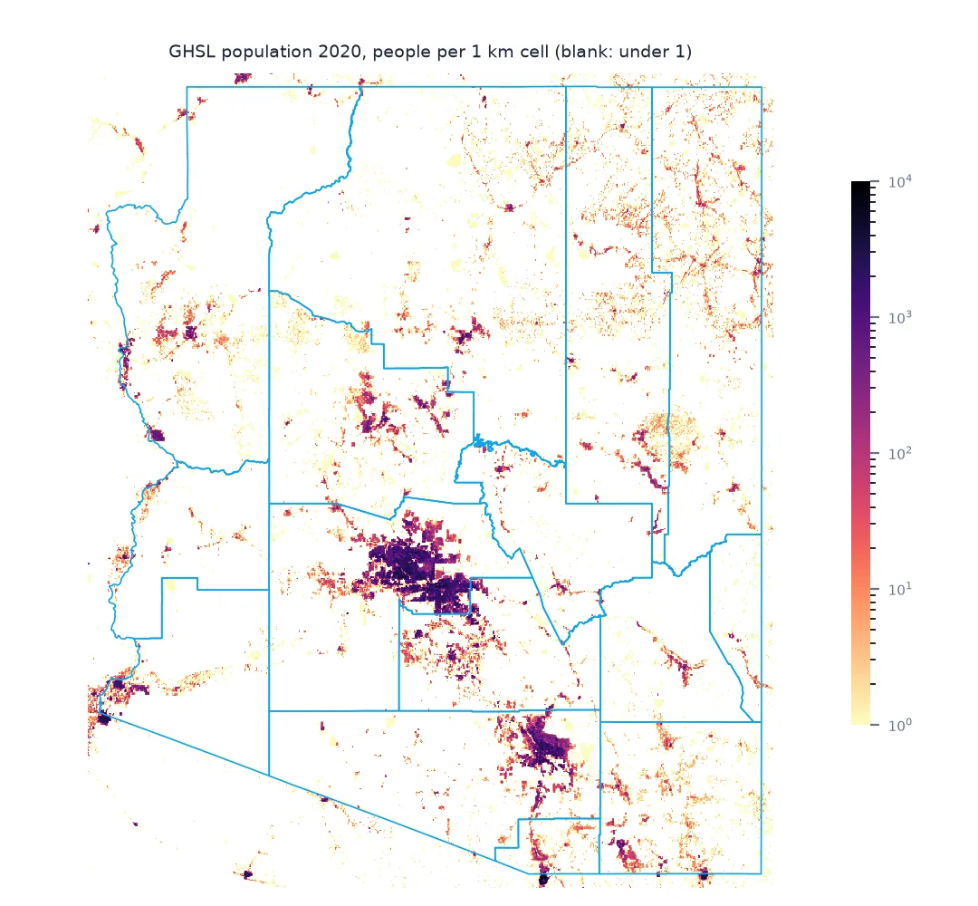
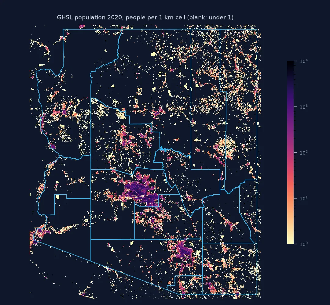
The fix samples grid cells in proportion to their population, so a cell with 5,000 people is 5,000 times as likely to receive a dot as a cell with one. The dots then follow settlements, road corridors and suburbs. The quick answer's weighted placement leaves almost no dots in empty cells.

Weighting changes more than the empty cells. In Pima, Pinal and Yavapai counties the busiest 5% of cells hold more than 95% of the people, so their dots now cluster in Tucson, the Phoenix suburbs and Prescott instead of covering the county evenly.

3. Keep jittered dots inside their county

Jittering inside a 1 km cell can push a dot across a county line when the cell straddles it. Count and redraw:

inside = np.concatenate([shapely.contains_xy(g, *pts.T) for g, pts in
                         zip(az.geometry, np.split(W, np.cumsum([int(round(v / 1000)) for v in az.total_votes])[:-1]))])
print(f"{(~inside).sum()} of {len(W):,} weighted dots fell outside their own county")

def weighted_points_inside(geom, n, rng):
    pts = np.empty((0, 2))
    while len(pts) < n:
        p = weighted_points(geom, n, rng)
        pts = np.vstack([pts, p[shapely.contains_xy(geom, *p.T)]])
    return pts[:n]

check = weighted_points_inside(az.geometry.iloc[0], 500, rng)
print("after rejection:", shapely.contains_xy(az.geometry.iloc[0], *check.T).all())

2 of 3,389 weighted dots fell outside their own county
after rejection: True

4. Check the grid against the census

A population grid is a model, built by distributing census counts over built-up areas. Its totals are close to the census but not equal:

ghsl = sum(np.maximum(mask(pop, [g], crop=True, nodata=0)[0][0], 0).sum() for g in az.geometry)
print(f"GHSL 2020 in Arizona's counties: {ghsl:,.0f}; Census 2020 apportionment population: {CENSUS_AZ:,}  "
      f"({ghsl / CENSUS_AZ - 1:+.1%})")

GHSL 2020 in Arizona's counties: 7,484,836; Census 2020 apportionment population: 7,158,923  (+4.6%)

For dot placement only the relative weights within each county matter, so a few percent of total error does not move dots. For anything that adds dots across counties, use the official counts and the grid only for placement.

Residents are not voters

The data used on this page

2024 presidential results by county from tonmcg/US_County_Level_Election_Results_08-24; Arizona counties from the US Census Bureau cartographic boundary files, 2023, 1:500,000; GHS-POP R2023A for 2020 at 30 arc-seconds, tiles R6_C7 and R6_C8 (European Commission JRC); the Census Bureau's 2020 apportionment table for Arizona's population.

import zipfile
from pathlib import Path

import geopandas as gpd
import numpy as np
import pandas as pd
import rasterio
import requests
import shapely
from rasterio.mask import mask
from rasterio.merge import merge

Path("data").mkdir(exist_ok=True)
GHS = ("https://jeodpp.jrc.ec.europa.eu/ftp/jrc-opendata/GHSL/GHS_POP_GLOBE_R2023A/GHS_POP_E2020_GLOBE_R2023A_4326_30ss/V1-0/tiles/"
       "GHS_POP_E2020_GLOBE_R2023A_4326_30ss_V1_0_R6_C{}.zip")
SOURCES = {"2024_US_County_Level_Presidential_Results.csv": "https://raw.githubusercontent.com/tonmcg/US_County_Level_Election_Results_08-24/master/2024_US_County_Level_Presidential_Results.csv",
           "cb_2023_us_county_500k.zip": "https://www2.census.gov/geo/tiger/GENZ2023/shp/cb_2023_us_county_500k.zip",
           "apportionment-2020-table01.xlsx": "https://www2.census.gov/programs-surveys/decennial/2020/data/apportionment/apportionment-2020-table01.xlsx",
           "ghs_R6_C7.zip": GHS.format(7), "ghs_R6_C8.zip": GHS.format(8)}
for name, url in SOURCES.items():
    if not Path("data", name).exists():
        Path("data", name).write_bytes(requests.get(url, timeout=600).content)
tiles = []
for c in (7, 8):
    tif = f"GHS_POP_E2020_GLOBE_R2023A_4326_30ss_V1_0_R6_C{c}.tif"
    if not Path("data", tif).exists():
        zipfile.ZipFile(f"data/ghs_R6_C{c}.zip").extract(tif, "data")
    tiles.append(rasterio.open(Path("data", tif)))
arr, tr = merge(tiles, bounds=(-115.0, 31.2, -108.9, 37.1))
with rasterio.open("data/ghs_pop_arizona.tif", "w", **(tiles[0].profile | {"height": arr.shape[1], "width": arr.shape[2], "transform": tr})) as dst:
    dst.write(arr)
pop = rasterio.open("data/ghs_pop_arizona.tif")
res = pd.read_csv("data/2024_US_County_Level_Presidential_Results.csv", dtype={"county_fips": str}).set_index("county_fips")
az = gpd.read_file("data/cb_2023_us_county_500k.zip").query("STATEFP == '04'").to_crs(4326).reset_index(drop=True)
az = az.join(res[["votes_gop", "votes_dem", "total_votes"]], on="GEOID")
seats = pd.read_excel("data/apportionment-2020-table01.xlsx", header=None)
CENSUS_AZ = int(seats[seats[0] == "Arizona"].iloc[0, 1])


def uniform_points(geom, n, rng):
    pts = np.empty((0, 2)); x0, y0, x1, y1 = geom.bounds
    while len(pts) < n:
        x, y = rng.uniform(x0, x1, 3 * n + 10), rng.uniform(y0, y1, 3 * n + 10)
        pts = np.vstack([pts, np.c_[x, y][shapely.contains_xy(geom, x, y)]])
    return pts[:n]


def residents_at(pts):
    return np.array([v[0] for v in pop.sample(map(tuple, pts))])


print(f"{len(az)} counties; grid {pop.width} x {pop.height}; Arizona census 2020: {CENSUS_AZ:,}")

15 counties; grid 732 x 708; Arizona census 2020: 7,158,923

Example 1: residents are not voters

share = []
for _, cty in az.iterrows():
    people = np.maximum(mask(pop, [cty.geometry], crop=True, nodata=0)[0][0], 0).sum()
    share.append((cty.NAME, cty.total_votes / people))
s = pd.DataFrame(share, columns=["county", "votes per resident"]).sort_values("votes per resident")
print(s.iloc[[0, 1, -2, -1]].round(2).to_string(index=False))

    county  votes per resident
      Yuma                0.35
Santa Cruz                0.41
    Mohave                0.56
   Yavapai                0.72

Votes per resident vary by county, through age structure, registration and turnout. Weighting by residents puts dots where people live; it cannot know which of them voted. Within a county, that error is invisible; between counties, the dot counts come from the votes, so it does not arise.

What a dot claims

A dot on a dot-density map claims "votes were cast around here". Uniform placement can only honour the "inside this county" part of that claim. Dasymetric placement uses ancillary data on where people are, such as a population grid, building footprints or land cover, to restrict the dots to plausible locations. It is the same idea as dasymetric mapping of population, applied to random points.

The ancillary data brings its own assumptions. A 2020 grid is not 2024. A grid built from building footprints can miss new subdivisions and count empty second homes. Its cell size limits how precisely dots can sit. Those errors are small compared with spreading Maricopa County's two million votes evenly over a county where four cells in five have no resident at all. Either way the map should state what it used.

Lakes, tribal lands and random seeds

• Lakes and reservoirs inside county polygons receive no dots under weighting, since nobody lives on them.
• Tribal lands with dispersed settlement get fewer, scattered dots; that reflects the population grid.
• Finer grids (100 m GHSL, census blocks) place dots more precisely but cost more memory.
• Fix the random seed so the map does not change every run.
• Rejection sampling for border cells is cheap; there are very few such dots.
• Never present the dots as locations; label the map with the dot value and the placement method.

Internal links

• How to make a dot-density election map — the whole recipe
• How to make a US county election map — the data
• Dasymetric mapping in Python — the same idea for population

FAQ

Why are the dots on my dot density map in empty areas?

Because they were placed uniformly at random inside each polygon; weight placement by a population grid instead.

What population data can I use to place dots?

The GHSL GHS-POP grid (global, 100 m to 1 km), WorldPop, or census blocks where available; all are free.

How many dots end up in empty land with uniform placement?

In Arizona's 2024 presidential vote, about 84% of dots fell in 1 km cells with under one resident; with population weighting, almost none.

Can weighted dots cross county lines?

Yes, when jittered within a border cell; reject and redraw them. In Arizona it affected well under 1% of dots.