
How to Make a Contiguous Cartogram in Python
On this page
Problem statement
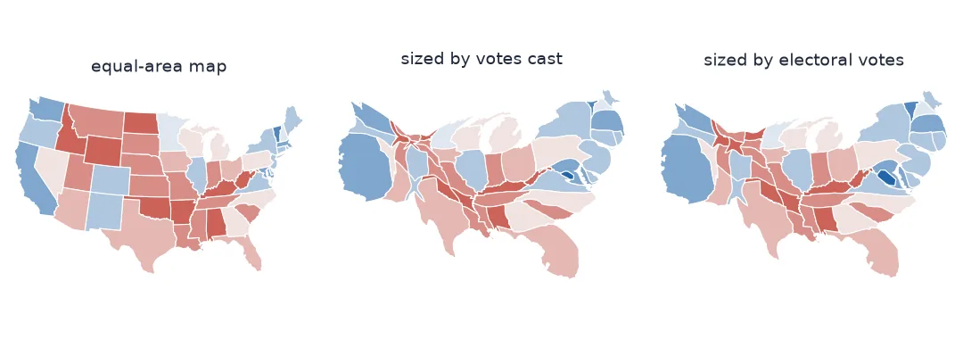
On an ordinary map, area is land. For anything measured in people — votes, population, cases, income — that hands the visual weight to the emptiest places: Wyoming cast 0.17% of the 2024 presidential vote in the lower 48 and covers 3.2% of the map; New Jersey cast 2.8% and covers 0.26%. A contiguous cartogram fixes this by reshaping every region until its area is proportional to the quantity, while keeping neighbours touching so the map is still recognisable.
There is no cartogram function in GeoPandas. This page implements the classic algorithm of Dougenik, Chrisman and Niemeyer (1985) in about 25 lines of NumPy and Shapely. It applies the algorithm to the 48 contiguous states and DC, sized first by votes cast in 2024 and then by electoral votes, and measures how close the result gets and what it costs in shape.
Quick answer
Iteratively push every vertex away from regions that are too small and towards regions that are too large, with forces that fall off with distance:
def cartogram(geoms, values, iterations=12):
    geoms, values, history = np.array(geoms, dtype=object), np.asarray(values, float), []
    for _ in range(iterations):
        area = shapely.area(geoms)
        desired = values / values.sum() * area.sum()
        centre = shapely.get_coordinates(shapely.centroid(geoms))
        radius = np.sqrt(area / np.pi)
        mass = np.sqrt(desired / np.pi) - radius                          # > 0: region must grow
        size_error = np.maximum(area, desired) / np.minimum(area, desired)
        history.append(size_error.mean())
        reduce = 1 / (1 + size_error.mean())                              # damping
        xy = shapely.get_coordinates(geoms)
        shift = np.zeros_like(xy)
        for k in range(len(geoms)):
            d = xy - centre[k]
            dist = np.maximum(np.hypot(d[:, 0], d[:, 1]), 1e-9)
            force = np.where(dist > radius[k], mass[k] * radius[k] / dist,
                             mass[k] * (dist / radius[k]) ** 2 * (4 - 3 * dist / radius[k]))
            shift += d / dist[:, None] * (force * reduce)[:, None]
        geoms = shapely.set_coordinates(geoms.copy(), xy + shift)
    return geoms, history

shaped, history = cartogram(states.geometry.values, states.total_votes.values)
print("mean size error by pass:", [round(float(h), 2) for h in history])
mean size error by pass: [5.54, 3.31, 2.43, 1.9, 1.55, 1.34, 1.21, 1.13, 1.09, 1.06, 1.04, 1.03]
Prepare regions, understand the forces, iterate and check
1. Prepare the regions and the values
Work in an equal-area projection, so the starting areas mean something, and drop regions that are not connected to the rest (Alaska and Hawaii are handled separately, or as insets):
print(f"{len(states)} regions in EPSG:5070; {states.total_votes.sum():,} votes; "
      f"{len(shapely.get_coordinates(states.geometry.values)):,} vertices")
share = states.assign(land=states.area / states.area.sum(), votes=states.total_votes / states.total_votes.sum())
print(share.set_index("STUSPS").loc[["WY", "NJ", "CA", "TX", "RI"], ["land", "votes"]].round(4).to_string())
49 regions in EPSG:5070; 154,022,941 votes; 11,058 vertices
land votes
STUSPS
WY 0.0323 0.0017
NJ 0.0026 0.0277
CA 0.0524 0.1030
TX 0.0884 0.0739
RI 0.0004 0.0033
2. Understand the forces
Each region is treated as a circle of its current area. Its "mass" is the difference between the radius it should have and the radius it has. Every vertex on the map — not only the region's own — is pushed outward from a region that must grow, and pulled inward towards one that must shrink. Outside the circle the force falls off as radius over distance. Inside it follows a smooth polynomial, so vertices near a centroid do not fly apart. All the forces are added up and applied together, damped by the average size error.
Because the shift depends only on a vertex's position, two neighbours' copies of a shared border vertex move identically. That is what keeps the map contiguous without any topology handling.
3. Iterate and watch the error
area = shapely.area(shaped)
target = states.total_votes.values / states.total_votes.sum()
miss = np.abs(area / area.sum() - target) / target
print(f"after {len(history)} passes: median area error {np.median(miss):.1%}, worst {miss.max():.1%} "
      f"({states.STUSPS.values[miss.argmax()]})")
print(f"valid geometries: {shapely.is_valid(shaped).sum()} of {len(shaped)}")
for n in (20, 30):
    g, _ = cartogram(states.geometry.values, states.total_votes.values, n)
    m = np.abs(shapely.area(g) / shapely.area(g).sum() - target) / target
    print(f"{n} passes: worst {m.max():.1%} ({states.STUSPS.values[m.argmax()]}), median {np.median(m):.2%}")
after 12 passes: median area error 0.7%, worst 18.7% (MT)
valid geometries: 49 of 49
20 passes: worst 4.9% (MT), median 0.05%
30 passes: worst 1.5% (MT), median 0.01%
The error falls fast at first and slowly after that. A dozen passes is usually enough for a national map. More passes keep shrinking the error but twist the shapes further.
Montana is the worst fit after twelve passes, 18.7% off its target: it has to shrink to a tenth of its land area, the second-largest reduction after Wyoming's. Twenty passes bring it within 5%, thirty within 2%.
4. Check that neighbours still touch
def neighbours(geoms):
    tree = shapely.STRtree(geoms)
    a, b = tree.query(geoms, predicate="intersects")
    return {(i, j) for i, j in zip(a, b) if i < j}

before, after = neighbours(states.geometry.values), neighbours(shaped)
print(f"neighbour pairs: {len(before)} before, {len(after)} after; lost {len(before - after)}, gained {len(after - before)}")
neighbour pairs: 109 before, 109 after; lost 0, gained 0
5. Size by a different quantity
The same function sizes the map by electoral votes, which is what decides the presidency:
print(f"48 states + DC: {states.ev.sum()} electoral votes (538 minus Alaska's 3 and Hawaii's 4 = 531)")
shaped_ev, history_ev = cartogram(states.geometry.values, states.ev.values)
area_ev = shapely.area(shaped_ev)
print(f"final mean size error {history_ev[-1]:.3f}")
red = states.margin > 0
for label, a in (("land", states.area.values), ("votes cast", shapely.area(shaped)), ("electoral votes", area_ev)):
    print(f"{label:16s}: {a[red].sum() / a.sum():.0%} of the map is Republican-won")
48 states + DC: 531 electoral votes (538 minus Alaska's 3 and Hawaii's 4 = 531)
final mean size error 1.015
land : 71% of the map is Republican-won
votes cast : 59% of the map is Republican-won
electoral votes : 58% of the map is Republican-won
Which states change most
The data used on this page
2024 presidential results by county from tonmcg/US_County_Level_Election_Results_08-24, summed to states; state boundaries from the US Census Bureau cartographic boundary files, 2023, 1:20 million; House seats from the Census Bureau's 2020 apportionment table.
from pathlib import Path

import geopandas as gpd
import numpy as np
import pandas as pd
import requests
import shapely

Path("data").mkdir(exist_ok=True)
SOURCES = {
    "2024_US_County_Level_Presidential_Results.csv": "https://raw.githubusercontent.com/tonmcg/US_County_Level_Election_Results_08-24/master/2024_US_County_Level_Presidential_Results.csv",
    "cb_2023_us_state_20m.zip": "https://www2.census.gov/geo/tiger/GENZ2023/shp/cb_2023_us_state_20m.zip",
    "apportionment-2020-table01.xlsx": "https://www2.census.gov/programs-surveys/decennial/2020/data/apportionment/apportionment-2020-table01.xlsx",
}
for name, url in SOURCES.items():
    if not Path("data", name).exists():
        Path("data", name).write_bytes(requests.get(url, timeout=300).content)
states = gpd.read_file("data/cb_2023_us_state_20m.zip")
states = states[~states.STUSPS.isin(["AK", "HI", "PR"])].to_crs(5070).reset_index(drop=True)
res = pd.read_csv("data/2024_US_County_Level_Presidential_Results.csv", dtype={"county_fips": str})
states = states.join(res.groupby(res.county_fips.str[:2])[["votes_gop", "votes_dem", "total_votes"]].sum(), on="STATEFP")
states["margin"] = (states.votes_gop - states.votes_dem) / states.total_votes
seats = pd.read_excel("data/apportionment-2020-table01.xlsx", header=None).iloc[4:54, [0, 2]]
ev = dict(zip(seats[0], seats[2].astype(int) + 2)) | {"District of Columbia": 3}    # senators + representatives
states["ev"] = states.NAME.map(ev)
print(f"{len(states)} regions; electoral votes for all 50 states + DC: {sum(ev.values())}")
49 regions; electoral votes for all 50 states + DC: 538
Example 1: which states change most
grow = pd.DataFrame({"state": states.STUSPS, "land %": states.area / states.area.sum() * 100,
                     "cartogram %": shapely.area(shaped) / shapely.area(shaped).sum() * 100})
grow["factor"] = grow["cartogram %"] / grow["land %"]
print(grow.sort_values("factor").iloc[[0, 1, 2, -3, -2, -1]].round(2).to_string(index=False))
state land % cartogram % factor
WY 3.23 0.18 0.06
MT 4.86 0.46 0.10
ND 2.34 0.25 0.11
RI 0.04 0.33 8.12
NJ 0.26 2.76 10.70
DC 0.00 0.23 101.86
Example 2: save it for a web map
out = gpd.GeoDataFrame(states[["STUSPS", "margin", "total_votes", "ev"]], geometry=list(shaped), crs=5070)
out.to_crs(4326).to_file("data/cartogram_votes_2024.geojson", driver="GeoJSON")
print(f"{Path('data/cartogram_votes_2024.geojson').stat().st_size / 1e3:.0f} kB; note: the coordinates are no longer geography")
508 kB; note: the coordinates are no longer geography
Exported cartogram coordinates are not real places. Label the file and the map as a cartogram, and never use it for distance, area or overlay.
Trading shape for size
A contiguous cartogram trades shape for size. Every algorithm has to give somewhere: Dougenik-Chrisman-Niemeyer moves boundaries with distance-decaying forces. Gastner-Newman diffusion lets density flow like a gas until it is even. Rubber-sheet and fast-flow methods are refinements of the same idea. All of them keep topology and give up exact shapes. The worse the mismatch between land and value, the harder they have to twist.
For US elections the mismatch is large in both directions. Small, dense places have to swell many times over — New Jersey nearly elevenfold, DC a hundredfold — and empty western states shrink to slivers: Wyoming to a seventeenth of its area. The result is less pleasing than a map, and more honest about what was decided where. Sizing by electoral votes, which give every state at least three, changes the colour balance surprisingly little: 58% of the map is Republican-won, against 59% by votes cast and 71% by land.
Islands, too many passes and vertex density
- Islands and exclaves (Michigan's two peninsulas, Hawaii) move as separate parts of one region; keep them in one multipolygon.
- Too many passes keep twisting shapes for little gain; stop when the mean size error is near 1.0.
- Vertex density matters: a 1:20m state outline has too few vertices to bend smoothly in tight places; densify first for county maps.
- Zero values cannot become zero area; give them a small floor or leave them out.
- The algorithm is O(regions × vertices) per pass; thousands of counties take seconds to minutes in NumPy.
- Always show a normal map alongside; readers navigate a cartogram by the shapes they already know.
Internal links
- How to make a US county election map — the map this corrects
- Choropleth maps in GeoPandas — the colouring
- Choosing a projected CRS — start from equal area
FAQ
How do I make a cartogram in Python?
Implement an iterative algorithm such as Dougenik-Chrisman-Niemeyer with NumPy and Shapely (as above), or use a diffusion-based package; GeoPandas has no built-in cartogram.
What is a contiguous cartogram?
A map where each region's area is proportional to a value while neighbouring regions still share borders, at the cost of distorted shapes.
How many iterations does a cartogram need?
For US states, about a dozen passes bring the mean size error close to 1; more passes give little improvement and more distortion.
Why does my cartogram look twisted?
Large mismatches between land area and value force strong distortions; very small or very large values relative to land create the worst twists.