Origin–Destination Data Explained

Problem statement

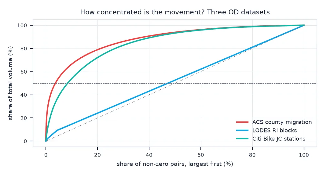
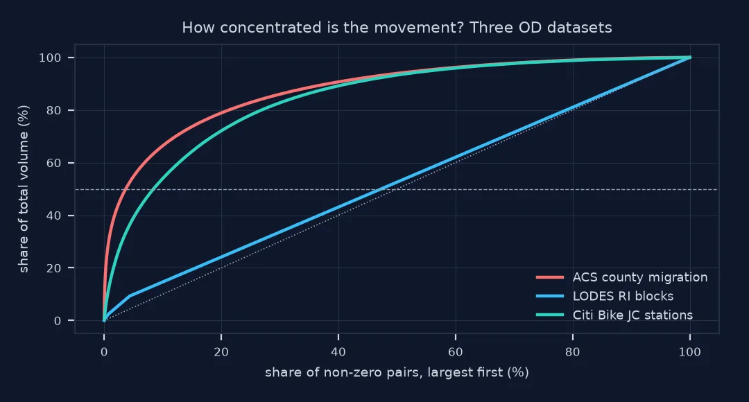
Origin–destination (OD) data records movement as pairs: from here, to there, how many. It is behind every flow map, transport model and migration study. It comes from very different sources: national surveys, administrative records and the logs of a bike-share system. They share a shape but not their properties. Some are samples with margins of error; others are complete counts with noise added for privacy. Some are tallies of people, others of jobs or trips. And almost all are extremely sparse, with most possible pairs empty. How concentrated the movement is depends on the zones: at county level a few pairs carry most of it, at block level almost none do.

This page sets out what an OD dataset is and how to describe one. It measures three real datasets used in this topic's guides: Census migration flows, LODES commuting, and Citi Bike trips.

Quick answer

Describe any OD dataset by its unit, its zones, its direction and how it was collected. Then measure two things before mapping it: how many of the possible pairs have any flow (sparsity), and how much of the volume the largest pairs carry (concentration):

def describe(name, o, d, v):
    pairs = pd.DataFrame({"o": o, "d": d, "v": v}).groupby(["o", "d"]).v.sum()
    zones = len(set(o) | set(d))
    s = pairs.sort_values(ascending=False)
    top1 = s.iloc[: max(1, len(s) // 100)].sum() / s.sum()
    print(f"{name:26s}: {zones:>6,} zones, {len(pairs):>9,} non-zero pairs = {len(pairs) / zones ** 2:.4%} of possible; "
          f"top 1% of pairs carry {top1:.0%}")

for name, (o, d, v) in DATA.items():
    describe(name, o, d, v)

ACS county migration      :  3,221 zones,   254,348 non-zero pairs = 2.4516% of possible; top 1% of pairs carry 33%
LODES RI blocks           : 21,890 zones,   360,924 non-zero pairs = 0.0753% of possible; top 1% of pairs carry 3%
Citi Bike JC stations     :    273 zones,     5,802 non-zero pairs = 7.7849% of possible; top 1% of pairs carry 15%

The unit, the direction, the diagonal and collection

1. Know the unit

The same "flow" means different things. ACS migration flows count people who moved, estimated from a sample. LODES counts jobs, so a person with two jobs appears twice. A bike-share log counts trips, so one person can appear dozens of times a month:

for name, (o, d, v) in DATA.items():
    print(f"{name:26s}: total {v.sum():>12,.0f} {UNIT[name]}")

ACS county migration      : total   18,061,885 movers (5 years)
LODES RI blocks           : total      380,586 jobs
Citi Bike JC stations     : total      110,673 trips (1 month)

2. Know the direction and the diagonal

All three are directed: A → B and B → A are different rows. All three can have a diagonal, flows from a zone to itself, but they treat it differently. The ACS county file leaves out moves within a county, LODES includes people working in their home block, and bike share records round trips:

for name, (o, d, v) in DATA.items():
    diag = v[np.asarray(o) == np.asarray(d)].sum()
    print(f"{name:26s}: diagonal {diag / v.sum():.1%} of the total")

ACS county migration      : diagonal 0.0% of the total
LODES RI blocks           : diagonal 0.1% of the total
Citi Bike JC stations     : diagonal 5.1% of the total

3. Know how it was collected

The collection method decides which numbers can be trusted. A survey such as the ACS has sampling error, published as margins of error, which make small flows unreliable. Administrative data such as LODES is a near-complete count with deliberate noise in small cells. A system log such as bike-share trips is exact but covers only its own system's users. Each needs a different check before mapping: margins of error, aggregation, or a statement of coverage.

A concentration curve of county flows

The data used on this page

The Census Bureau's county-to-county migration flows, 2016–2020 ACS; LODES version 8 commuting for Rhode Island, 2021 (main, all jobs, block to block); and Citi Bike trips in Jersey City and Hoboken, June 2024 (station to station).

import zipfile
from pathlib import Path

import numpy as np
import pandas as pd
import requests

Path("data").mkdir(exist_ok=True)
SRC = {"county-to-county-2016-2020-ins-outs-nets-gross.xlsx": "https://www2.census.gov/programs-surveys/demo/tables/geographic-mobility/2020/"
       "county-to-county-migration-2016-2020/county-to-county-migration-flows/county-to-county-2016-2020-ins-outs-nets-gross.xlsx",
       "ri_od_main_JT00_2021.csv.gz": "https://lehd.ces.census.gov/data/lodes/LODES8/ri/od/ri_od_main_JT00_2021.csv.gz",
       "JC-202406-citibike-tripdata.csv.zip": "https://s3.amazonaws.com/tripdata/JC-202406-citibike-tripdata.csv.zip"}
for name, url in SRC.items():
    if not Path("data", name).exists():
        Path("data", name).write_bytes(requests.get(url, timeout=600).content)
COLS = ["a_st", "a_cty", "b_st", "b_cty", "a_state", "a_county", "b_state", "b_county",
        "flow", "flow_moe", "counter", "counter_moe", "net", "net_moe", "gross", "gross_moe"]
mig = pd.concat(pd.read_excel("data/county-to-county-2016-2020-ins-outs-nets-gross.xlsx", sheet_name=None, header=None,
                              skiprows=3, names=COLS, dtype=str).values())
mig = mig[mig.a_cty.notna() & mig.b_st.str.fullmatch(r"\d{3}", na=False)]
mig_v = pd.to_numeric(mig.flow, errors="coerce").fillna(0)
mig = mig[mig_v > 0]; mig_v = mig_v[mig_v > 0]
lodes = pd.read_csv("data/ri_od_main_JT00_2021.csv.gz", dtype={"w_geocode": str, "h_geocode": str})
with zipfile.ZipFile("data/JC-202406-citibike-tripdata.csv.zip") as z:
    bike = pd.read_csv(z.open("JC-202406-citibike-tripdata.csv"), dtype={"start_station_id": str, "end_station_id": str},
                       usecols=["start_station_id", "end_station_id"]).dropna()
DATA = {"ACS county migration": ((mig.b_st.str[1:] + mig.b_cty).to_numpy(), (mig.a_st.str[1:] + mig.a_cty).to_numpy(), mig_v.to_numpy()),
        "LODES RI blocks": (lodes.h_geocode.to_numpy(), lodes.w_geocode.to_numpy(), lodes.S000.to_numpy()),
        "Citi Bike JC stations": (bike.start_station_id.to_numpy(), bike.end_station_id.to_numpy(), np.ones(len(bike)))}
UNIT = {"ACS county migration": "movers (5 years)", "LODES RI blocks": "jobs", "Citi Bike JC stations": "trips (1 month)"}
print({k: f"{len(v[2]):,} rows" for k, v in DATA.items()})

{'ACS county migration': '254,348 rows', 'LODES RI blocks': '360,924 rows', 'Citi Bike JC stations': '110,673 rows'}

Example 1: a concentration curve

curves = {}
for name, (o, d, v) in DATA.items():
    s = pd.DataFrame({"o": o, "d": d, "v": v}).groupby(["o", "d"]).v.sum().sort_values(ascending=False)
    curves[name] = (np.arange(1, len(s) + 1) / len(s), s.cumsum().to_numpy() / s.sum())
for name, (x, y) in curves.items():
    print(f"{name:26s}: pairs needed for half the volume: {x[np.searchsorted(y, 0.5)]:.1%}")

ACS county migration      : pairs needed for half the volume: 3.7%
LODES RI blocks           : pairs needed for half the volume: 47.3%
Citi Bike JC stations     : pairs needed for half the volume: 8.4%

A sparse matrix stored as pairs

Every OD dataset is a sparse matrix stored as a list of pairs. The sparsity is extreme: only 2.5% of possible county pairs in the US exchanged any movers in five years, and 0.08% of Rhode Island block pairs share a commuter. Concentration is a different matter and depends on the zones. Half of all county-to-county movers are in 3.7% of the county pairs, so a few dozen lines can tell most of the story. Half of Rhode Island's jobs are spread over 47% of the block pairs, nearly all of them holding a single job. At that level no flow map works until the blocks are aggregated.

The differences matter more than the shape. ACS flows are estimates with margins of error, so their small pairs are noise. LODES block pairs are near-complete but deliberately noisy in small cells, so they need aggregating. Citi Bike trips are exact counts of one system's users. A careful OD analysis starts by naming the unit, the zones, the direction, the period and the collection method, because those decide which of the steps in this topic's guides apply.

Zero pairs, symmetric storage and privacy

• Zero pairs are usually not stored; a missing pair means zero only if the source lists every non-zero pair.
• Symmetric storage: some files list each pair from both sides (the ACS workbook does); sum one direction only.
• Zone systems change over time (new counties, renumbered stations); OD tables from different years need a crosswalk.
• Privacy: fine-grained OD data can identify people; publishers suppress, perturb or synthesise small cells.
• Time: an OD table for a month, a year or five years describes a different process; state the period.

Internal links

• How to build an origin–destination matrix — the table form
• Flow maps explained — drawing OD data

FAQ

What is origin–destination data?

Counts of movement between pairs of places: from an origin zone, to a destination zone, how many people, jobs, trips or goods.

Where does OD data come from?

Surveys (such as the ACS migration flows), administrative records (such as LODES commuting), and system logs (such as bike-share trips or transit smart cards).

Why is OD data so sparse?

Most pairs of places never exchange anyone in a given period; the number of possible pairs grows with the square of the number of zones.

What should I check before mapping OD data?

The unit, direction and diagonal, the collection method and its uncertainty, sparsity, and how much of the volume the largest pairs carry.