How to Analyse Origin–Destination Flows by Hour of Day in Python

On this page

Problem statement

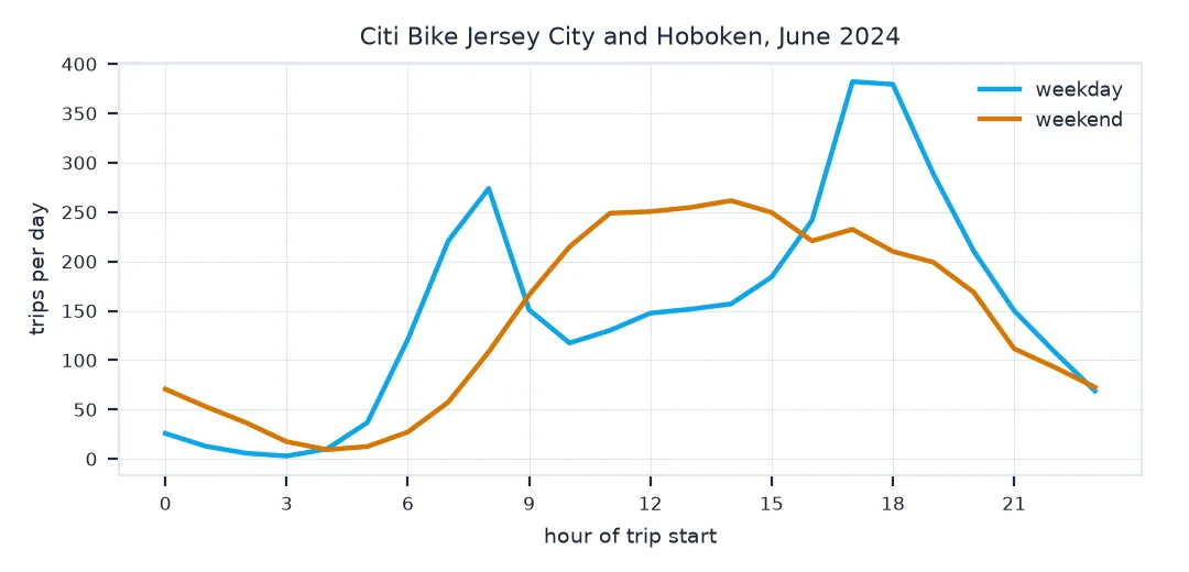
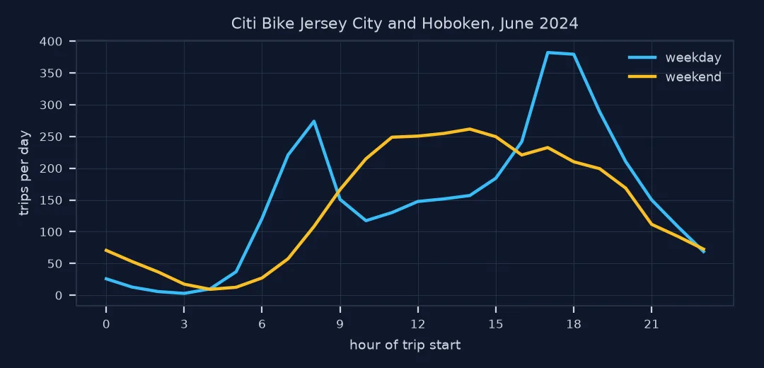
A flow map of a whole month shows where trips go, but not when. Most urban flows have a strong daily rhythm. Commuters ride towards the train in the morning and away from it in the evening, and leisure trips peak at weekends and in the afternoon. Adding time as a third dimension to an origin–destination table turns one map into a set of questions. Which routes are commuter routes? When does each direction peak? How different are weekdays and weekends? Answering them means grouping trips by hour and day type, normalising the profiles so routes of different size can be compared, and plotting them.

This page breaks a month of Citi Bike trips in Jersey City and Hoboken into hourly flows and compares a commuter route with a leisure route.

Quick answer

Add the hour and day type to each trip, then count trips per route per hour:

trips["hour"] = trips.started_at.dt.hour
trips["day"] = np.where(trips.started_at.dt.dayofweek < 5, "weekday", "weekend")
hourly = trips.groupby(["start_station_id", "end_station_id", "day", "hour"]).size().rename("trips").reset_index()
days = trips.groupby("day").started_at.apply(lambda s: s.dt.date.nunique())
system = trips.groupby(["day", "hour"]).size().unstack(0).div(days)                 # trips per day, by hour
print(f"{days.to_dict()} days; busiest weekday hour {system.weekday.idxmax()}:00 ({system.weekday.max():.0f} trips/day), "
      f"busiest weekend hour {system.weekend.idxmax()}:00 ({system.weekend.max():.0f} trips/day)")

{'weekday': 20, 'weekend': 10} days; busiest weekday hour 17:00 (382 trips/day), busiest weekend hour 14:00 (262 trips/day)

Line chart of Citi Bike trips per day by hour in Jersey City and Hoboken in June 2024: weekdays have a morning peak of about 275 at 8:00 and a higher evening peak of 382 at 17:00; weekends have a broad plateau around 250 from 11:00 to 15:00. — Trips per day by start hour. Weekdays have two commuter peaks; weekends one broad afternoon hump.

Rates not totals, how peaked each route is, both directions

1. Compare rates, not totals

June 2024 had 20 weekdays and 10 weekend days, so totals favour weekdays twice over. Divide by the number of days of each type before comparing:

tot = trips.groupby("day").size()
print(f"total trips: weekday {tot.weekday:,}, weekend {tot.weekend:,}; per day: weekday {tot.weekday / days.weekday:,.0f}, "
      f"weekend {tot.weekend / days.weekend:,.0f}")

total trips: weekday 71,565, weekend 33,465; per day: weekday 3,578, weekend 3,346

Per day, a weekend day is nearly as busy as a weekday: 3,346 trips against 3,578. The weekday total is twice as large only because there are twice as many weekdays.

2. Measure how peaked each route is

A commuter route concentrates its trips in a few hours; a leisure route spreads them out. The share of a route's weekday trips that start in the 7–9 and 16–18 peaks separates them:

wk = hourly[hourly.day == "weekday"]
route = wk.groupby(["start_station_id", "end_station_id"]).trips.sum().rename("total").reset_index()
peak = wk[wk.hour.isin([7, 8, 9, 16, 17, 18])].groupby(["start_station_id", "end_station_id"]).trips.sum()
route = route.join(peak.rename("peak"), on=["start_station_id", "end_station_id"]).fillna(0)
route = route[route.total >= 100].assign(peak_share=lambda d: d.peak / d.total)
print(f"{len(route)} routes with 100+ weekday trips; peak share median {route.peak_share.median():.0%}, "
      f"range {route.peak_share.min():.0%}–{route.peak_share.max():.0%}")
most, least = route.nlargest(1, "peak_share").iloc[0], route.nsmallest(1, "peak_share").iloc[0]
print(f"most peaked:  {NAMES[most.start_station_id]} -> {NAMES[most.end_station_id]} ({most.peak_share:.0%} of {most.total:.0f})")
print(f"least peaked: {NAMES[least.start_station_id]} -> {NAMES[least.end_station_id]} ({least.peak_share:.0%} of {least.total:.0f})")

116 routes with 100+ weekday trips; peak share median 54%, range 12%–77%
most peaked:  Brunswick St -> Grove St PATH (77% of 248)
least peaked: City Hall -> Grove St PATH (12% of 112)

Bar chart of weekday trips by hour on one route: Brunswick Street to Grove Street PATH peaks at 8:00 with about 100 trips in June, while the reverse direction peaks at 17:00 with about 50. — The most peaked route: 76% of trips to the PATH station start before noon, 9% of trips back.

3. See both directions of one route

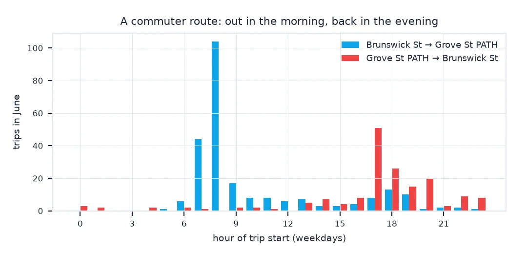
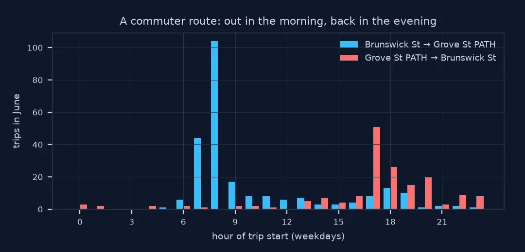
A commuter route's two directions peak at opposite ends of the day. Profile the busiest weekday route and its reverse:

a, b = most.start_station_id, most.end_station_id
there = wk[(wk.start_station_id == a) & (wk.end_station_id == b)].set_index("hour").trips.reindex(range(24), fill_value=0)
back = wk[(wk.start_station_id == b) & (wk.end_station_id == a)].set_index("hour").trips.reindex(range(24), fill_value=0)
print(f"{NAMES[a]} -> {NAMES[b]}: peak hour {there.idxmax()}:00; reverse: peak hour {back.idxmax()}:00")
print(f"share before noon: there {there[:12].sum() / there.sum():.0%}, back {back[:12].sum() / back.sum():.0%}")

Brunswick St -> Grove St PATH: peak hour 8:00; reverse: peak hour 17:00
share before noon: there 76%, back 9%

An hour-by-route matrix for plotting

The data used on this page

Citi Bike system data: Jersey City and Hoboken trips for June 2024 (JC-202406-citibike-tripdata). Times are local (New York time).

import zipfile
from pathlib import Path

import matplotlib
matplotlib.use("Agg")
import matplotlib.pyplot as plt
import numpy as np
import pandas as pd
import requests

Path("data").mkdir(exist_ok=True)
F = Path("data/JC-202406-citibike-tripdata.csv.zip")
if not F.exists():
    F.write_bytes(requests.get("https://s3.amazonaws.com/tripdata/" + F.name, timeout=600).content)
with zipfile.ZipFile(F) as z:
    trips = pd.read_csv(z.open("JC-202406-citibike-tripdata.csv"), parse_dates=["started_at"],
                        dtype={"start_station_id": str, "end_station_id": str})
trips = trips.dropna(subset=["start_station_id", "end_station_id"])
trips = trips[(trips.start_station_id != trips.end_station_id) & (trips.started_at.dt.month == 6)]   # the file also has trips from 31 May
NAMES = trips.groupby("start_station_id").start_station_name.first().to_dict()
NAMES.update(trips.groupby("end_station_id").end_station_name.first().to_dict())
print(f"{len(trips):,} trips between two stations, {trips.started_at.min():%d %b} to {trips.started_at.max():%d %b %Y}")

105,030 trips between two stations, 01 Jun to 30 Jun 2024

Example 1: an hour-by-route matrix for plotting

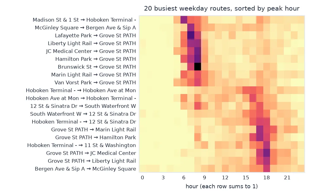
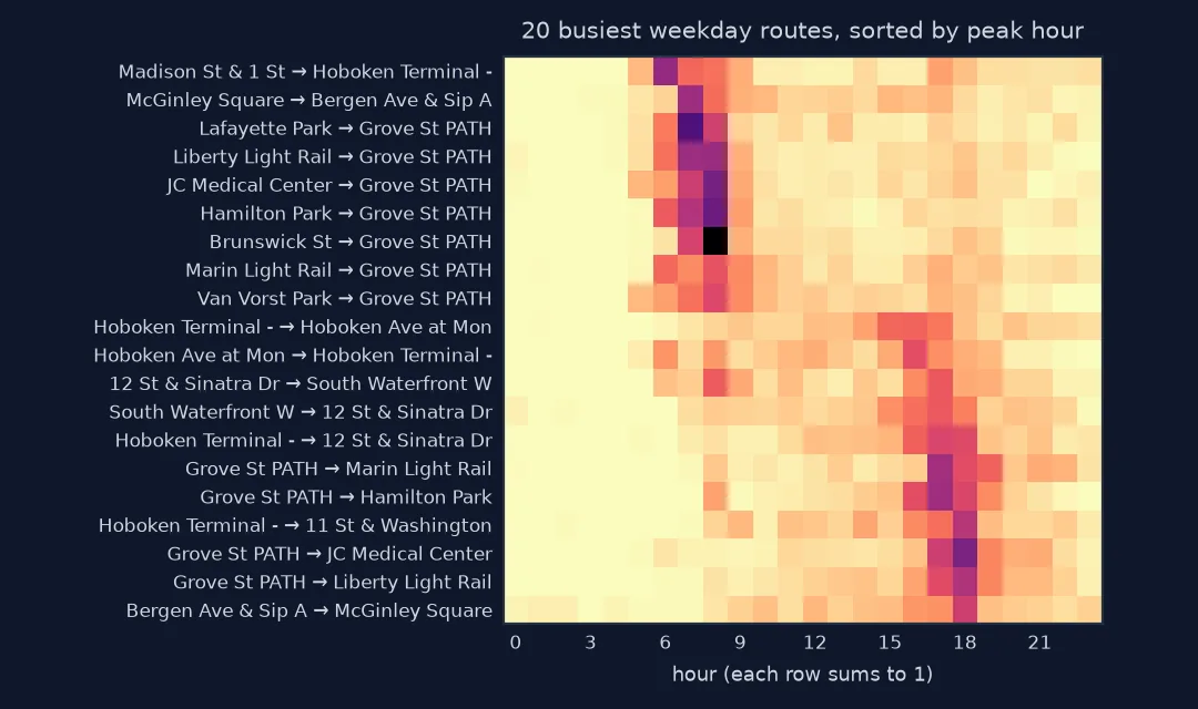
top_routes = route.nlargest(20, "total")
mat = np.array([wk[(wk.start_station_id == r.start_station_id) & (wk.end_station_id == r.end_station_id)]
                  .set_index("hour").trips.reindex(range(24), fill_value=0).to_numpy() for r in top_routes.itertuples()])
mat = mat / mat.sum(axis=1, keepdims=True)                                  # each row sums to 1: shape, not size
print(mat.shape, f"rows peaking before noon: {(mat.argmax(axis=1) < 12).sum()} of {len(mat)}")

(20, 24) rows peaking before noon: 9 of 20

A profile says what a route is for

Time-of-day analysis turns an origin–destination table into a set of profiles, one per route, and the shape of a profile says what the route is for. Commuter routes have two sharp peaks in opposite directions, morning out and evening back. Leisure routes have a broad afternoon hump, and on weekends the whole system shifts towards it. Normalising each profile to sum to one compares shapes rather than sizes, so a busy route does not dominate the picture.

Heatmap of the hourly profiles of the 20 busiest weekday routes, each row normalised and sorted by peak hour: routes into Grove Street PATH and Hoboken Terminal peak at 7 to 8 in the morning, routes out of them at 17 to 18, and waterfront routes in the late afternoon. — Each row is one route's weekday profile, scaled to sum to one, so shapes can be compared regardless of size.

Three practical points recur. Compare per-day rates, not totals, because months have unequal numbers of weekdays and weekend days. Keep the two directions of a route separate, since their peaks are often twelve hours apart. And set a minimum trip count before computing shares, because a route with five trips a month can have any shape at all.

Time zones, midnight trips and weather

Time-of-day problems and fixes.

Time zone: Citi Bike times are local; daylight-saving changes move one hour twice a year.
Trips over midnight are assigned to the start hour; use the end time for arrival profiles.
Holidays behave like weekend days; June 2024 had none in the US, but check other months.
Weather dominates day-to-day variation; a single month mixes rainy and dry days.
Small routes: set a minimum count (here 100 weekday trips) before computing shares.

Internal links

How to map bike-share trips as flows — the same trips as a map
How to build an origin–destination matrix — the table behind the flows

FAQ

How do I find peak hours in trip data with pandas?

Extract the hour with .dt.hour, group by it (and by route if needed), count, and divide by the number of days to get trips per day per hour.

How do I compare weekday and weekend trips fairly?

Divide counts by the number of weekdays and weekend days in the period, so you compare average days rather than totals.

How can I tell commuter routes from leisure routes?

Commuter routes concentrate their trips in the morning and evening peaks, with opposite directions peaking at opposite ends of the day; leisure routes spread trips across the afternoon.

Should I normalise hourly profiles?

To compare shapes between routes of different size, yes: divide each route's hourly counts by its total.