How to Aggregate Origin–Destination Flows to Larger Zones in Python

On this page

Problem statement

Flow data often comes at a finer level than the question. The Census county-to-county flows have more than 400,000 county pairs, most of them a few people with a margin of error larger than the estimate. A question about migration between states needs those pairs summed. Aggregating flows is a group-by, but three things change on the way up. Flows within the new zone become internal and leave the map. Margins of error must be combined, not added. And the result is more reliable but answers a different question.

This page sums the 2016–2020 county flows to state-to-state flows, propagates their margins of error, and measures how reliability changes with zone size.

Quick answer

Map each origin and destination to the larger zone, group, sum the estimates, and combine the MOEs as the square root of the sum of squares:

pairs = us.assign(o=us.b_st.str[1:], d=us.a_st.str[1:], m2=us.flow_moe ** 2)       # flow = moves from B (origin) into A
st = pairs.groupby(["o", "d"], as_index=False).agg(movers=("flow", "sum"), m2=("m2", "sum"))
st["moe"] = np.sqrt(st.m2)
inter = st[st.o != st.d]
print(f"{len(pairs):,} county pairs -> {len(st):,} state pairs ({len(inter):,} between different states); "
      f"interstate movers {inter.movers.sum():,.0f}, within-state {st.loc[st.o == st.d, 'movers'].sum():,.0f}")

406,348 county pairs -> 2,703 state pairs (2,652 between different states); interstate movers 7,542,146, within-state 10,519,739

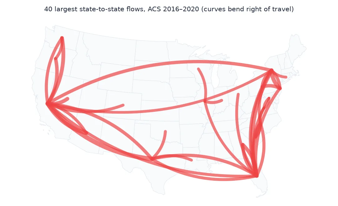
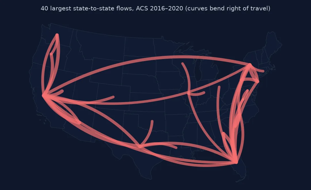
Flow map of the contiguous United States with 40 thick red curves for the largest state-to-state migration flows: a hub in California with flows to Texas, Arizona, Washington, Nevada and Oregon, a hub in Florida with flows from New York, New Jersey, Georgia and others, and flows from New York to New Jersey and from Illinois. — The 40 largest flows between states, summed from county pairs. Each is several tens of thousands of movers with a CV under 15%.

Each flow once, combined margins, compared reliability

1. Take each flow once

The workbook lists every county pair from both sides: the row for A = Los Angeles, B = Orange holds the same two numbers as the row for A = Orange, B = Los Angeles, swapped. Summing flow alone counts each directed move exactly once; summing flow and counter would count it twice:

mirror = us.merge(us, left_on=["a_st", "a_cty", "b_st", "b_cty"], right_on=["b_st", "b_cty", "a_st", "a_cty"], suffixes=("", "_m"))
print(f"rows whose flow equals the mirror row's counterflow: {(mirror.flow == mirror.counter_m).mean():.0%}")
print(f"sum of flow {us.flow.sum():,.0f} = sum of counter {us.counter.sum():,.0f}")

rows whose flow equals the mirror row's counterflow: 100%
sum of flow 18,061,885 = sum of counter 18,061,885

2. Combine the margins of error

Sampling errors partly cancel when estimates are added, so MOEs combine in quadrature. Adding them directly would overstate the uncertainty:

ny_fl = st[(st.o == "36") & (st.d == "12")].iloc[0]
added = pairs[(pairs.o == "36") & (pairs.d == "12")].flow_moe.sum()
print(f"New York -> Florida: {ny_fl.movers:,.0f} movers, MOE {ny_fl.moe:,.0f} (quadrature) vs {added:,.0f} (simple sum)")

New York -> Florida: 61,299 movers, MOE 3,364 (quadrature) vs 54,253 (simple sum)

The Census Bureau's quadrature formula assumes the estimates are independent. For flows within one survey that is an approximation, which is why it is called an approximate standard error.

3. Compare reliability at both levels

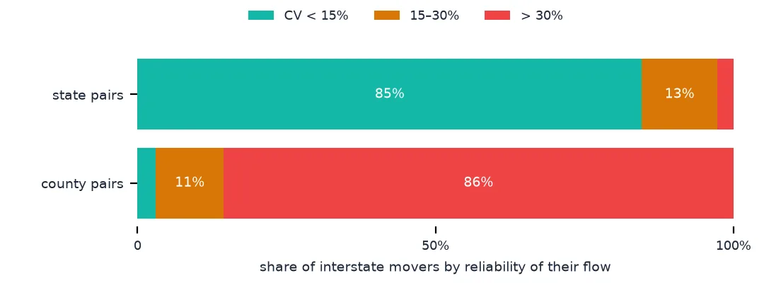
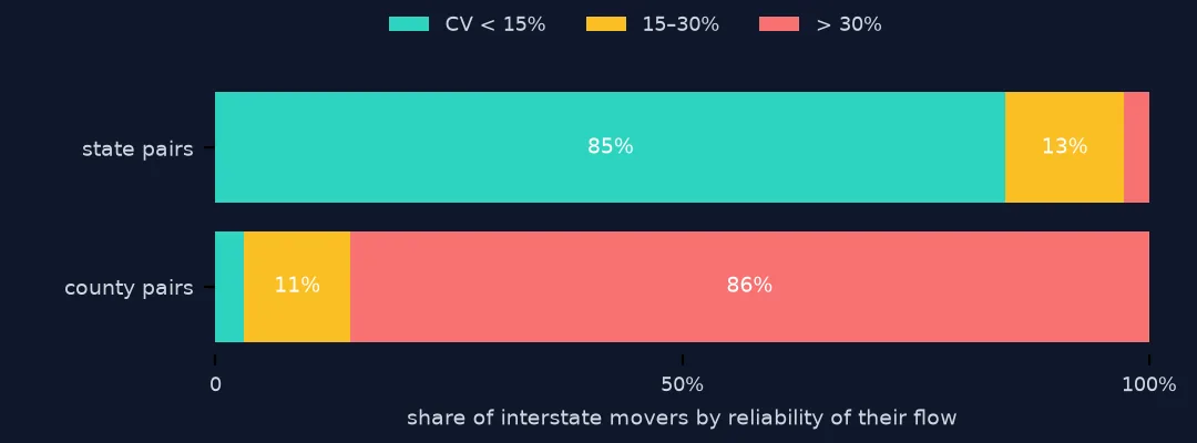
Aggregating trades detail for reliability. Compare the share of movers in reliable flows (CV under 15%) at the county and state levels:

def reliable_share(est, moe):
    cv = moe / 1.645 / est
    ok = est > 0
    return (est[ok & (cv < 0.15)]).sum() / est[ok].sum()

cty = pairs[pairs.o != pairs.d]                                            # interstate county pairs only, for a fair comparison
print(f"interstate movers in reliable flows: county pairs {reliable_share(cty.flow, cty.flow_moe):.0%}, "
      f"state pairs {reliable_share(inter.movers, inter.moe):.0%}")
print(f"state pairs with CV < 15%: {(inter.moe / 1.645 / inter.movers < 0.15).sum():,} of {len(inter):,}")

interstate movers in reliable flows: county pairs 3%, state pairs 85%
state pairs with CV < 15%: 828 of 2,652

Stacked bars of the share of interstate movers by reliability of their flow: at county-pair level 3% are in flows with a CV under 15% and 86% in flows over 30%; at state-pair level 85% are under 15% and very few over 30%. — The same movers, judged at two levels. Aggregating turns mostly unreliable county flows into mostly reliable state flows.

4. Rank the state-to-state flows

With the flows aggregated, the largest interstate moves can be ranked with confidence:

top = inter.nlargest(8, "movers").assign(o=lambda d: d.o.map(STATE), d=lambda d: d.d.map(STATE))
print(top[["o", "d", "movers", "moe"]].to_string(index=False, formatters={"movers": "{:,.0f}".format, "moe": "{:,.0f}".format}))

         o          d movers   moe
California      Texas 79,063 4,471
California    Arizona 64,625 3,365
  New York    Florida 61,299 3,364
  New York New Jersey 57,219 3,009
California Washington 51,213 2,633
California     Nevada 49,355 2,946
   Florida    Georgia 46,095 2,912
California     Oregon 43,222 2,526

The share of county moves that stay in the state

The data used on this page

The Census Bureau's county-to-county migration flows, 2016–2020 ACS (all 52 sheets of the "ins, outs, nets, gross" workbook) and the 2023 state cartographic boundary file.

from pathlib import Path

import geopandas as gpd
import matplotlib
matplotlib.use("Agg")
import matplotlib.pyplot as plt
import numpy as np
import pandas as pd
import requests

Path("data").mkdir(exist_ok=True)
SRC = {"county-to-county-2016-2020-ins-outs-nets-gross.xlsx": "https://www2.census.gov/programs-surveys/demo/tables/geographic-mobility/2020/"
       "county-to-county-migration-2016-2020/county-to-county-migration-flows/county-to-county-2016-2020-ins-outs-nets-gross.xlsx",
       "cb_2023_us_state_20m.zip": "https://www2.census.gov/geo/tiger/GENZ2023/shp/cb_2023_us_state_20m.zip"}
for name, url in SRC.items():
    if not Path("data", name).exists():
        Path("data", name).write_bytes(requests.get(url, timeout=600).content)
COLS = ["a_st", "a_cty", "b_st", "b_cty", "a_state", "a_county", "b_state", "b_county",
        "flow", "flow_moe", "counter", "counter_moe", "net", "net_moe", "gross", "gross_moe"]
sheets = pd.read_excel("data/county-to-county-2016-2020-ins-outs-nets-gross.xlsx", sheet_name=None, header=None,
                       skiprows=3, names=COLS, dtype=str)
flows = pd.concat(sheets.values())
flows = flows[flows.a_cty.notna() & flows.b_st.notna()].copy()
for c in COLS[8:]:
    flows[c] = pd.to_numeric(flows[c], errors="coerce")
us = flows[flows.b_st.str.fullmatch(r"\d{3}")]                       # US counties only, no foreign regions
us = us[us.flow.notna()].copy()
us["flow_moe"] = us.flow_moe.fillna(0)
STATES = gpd.read_file("data/cb_2023_us_state_20m.zip")
STATE = dict(zip(STATES.STATEFP, STATES.NAME))
print(f"{len(us):,} county-to-county rows between US counties")

406,348 county-to-county rows between US counties

out_of = st.groupby("o").movers.sum()
stay = st[st.o == st.d].set_index("o").movers / out_of
print(f"median share of moves to another county that stay in the state: {stay.median():.0%}; "
      f"lowest {STATE[stay.idxmin()]} {stay.min():.0%}, highest {STATE[stay.idxmax()]} {stay.max():.0%}")

median share of moves to another county that stay in the state: 57%; lowest Hawaii 12%, highest Texas 71%

Moves within one county are not county-to-county flows at all, so a state with few, large counties, such as Hawaii with five, keeps few of its flows inside the state.

A coarser question with more confidence

Aggregation answers a coarser question with more confidence. A county-to-county flow of 40 people between two rural counties says almost nothing on its own. Summed with thousands of similar flows into a state-to-state total, the noise largely cancels and the margin of error shrinks relative to the estimate. The same data, read at a level its sample size supports, becomes reliable.

Aggregation in numbers: 51 state pairs become internal and leave the flow map.

Two things change meaning on the way up. Moves within the new zone, such as from one Texas county to another, are no longer flows between zones; they become the diagonal and leave the flow map. And the zone boundaries now decide which moves count as "between": a move across a state line counts, a longer move within Texas does not. That is the modifiable areal unit problem in its flow form, and the reason a flow map should say which zones it uses.

Double counting, zero margins and foreign rows

Aggregation problems and fixes.

Double counting: sum one direction per row (flow here). The workbook holds every pair twice, once from each side.
MOE of zero: rows with a missing MOE (shown as blank) are treated as zero here; that slightly understates the aggregate MOE.
Approximate errors: the quadrature sum assumes independence; for publication-grade work use the ACS variance replicate tables where available.
Foreign rows are excluded; they have no counterflow and no US origin.
Puerto Rico is in the workbook with its own sheet; decide whether to include it in "US" totals.

Internal links

How to read county-to-county migration flows — the workbook and its columns
Why small flows are unreliable — margins of error at the county level

FAQ

How do I aggregate origin–destination data to larger zones?

Add columns for the larger origin and destination zones, group by them, and sum the counts. Flows within one larger zone become internal flows.

How do I combine margins of error when summing ACS estimates?

Take the square root of the sum of the squared MOEs. It is an approximation that assumes independent estimates.

Why are state-level flows more reliable than county-level flows?

Each state flow sums many county flows; their sampling errors partly cancel, so the MOE grows more slowly than the estimate.

Does aggregating flows change the result?

Yes: moves within the new zones disappear from the flows, and which moves count as "between zones" depends on where the boundaries are.