
Why Do Small Migration Flows Jump Around Between Releases?
On this page
Problem statement
You map county-to-county migration from one ACS release, then from the next, and the small flows have changed beyond recognition. A flow of 40 people is now 150, another of 90 is now zero. The large flows barely move. It looks like migration patterns shifted, but mostly they did not. A small flow rests on a handful of survey responses, and its margin of error is as large as the estimate. Two independent samples of the same small flow can differ several-fold by chance alone.
This page compares the flows out of Los Angeles County in two non-overlapping ACS releases, 2011–2015 and 2016–2020. It measures how much they change by size and tests which changes exceed their margins of error.
Quick answer
Before reading a change between releases, test it: compare the difference with the combined MOE of the two estimates.
both = a.merge(b, on="geoid", suffixes=("_15", "_20"))
both["change"] = both.movers_20 - both.movers_15
both["change_moe"] = np.sqrt(both.moe_15 ** 2 + both.moe_20 ** 2)
both["real"] = both.change.abs() > both.change_moe
print(f"{len(both):,} destinations in both releases; changes larger than their MOE: {both.real.sum():,} ({both.real.mean():.0%})")
885 destinations in both releases; changes larger than their MOE: 77 (9%)
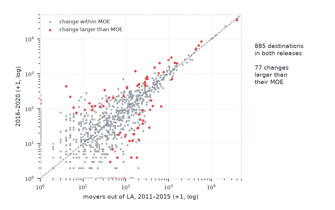
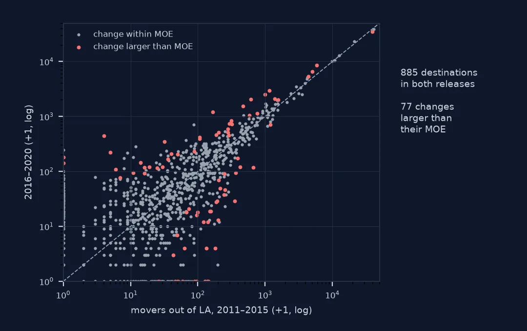
Swings by size, the margins themselves, what can be told apart
1. Measure the swings by size
Compare the ratio between the two releases for small and large flows:
both["size"] = pd.cut((both.movers_15 + both.movers_20) / 2, [0, 50, 200, 1000, 5000, np.inf],
                      labels=["<50", "50–200", "200–1k", "1k–5k", "5k+"])
both["ratio"] = (both.movers_20 + 1) / (both.movers_15 + 1)
summary = both.groupby("size", observed=True).agg(pairs=("ratio", "size"),
                                                  median_swing=("ratio", lambda r: np.median(np.abs(np.log2(r)))),
                                                  real_change=("real", "mean"))
summary["typical factor"] = 2 ** summary.median_swing
print(summary[["pairs", "typical factor", "real_change"]].to_string(formatters={"typical factor": "{:.2f}x".format, "real_change": "{:.0%}".format}))
pairs typical factor real_change
size
<50 474 3.71x 3%
50–200 235 2.19x 15%
200–1k 115 1.43x 17%
1k–5k 36 1.22x 19%
5k+ 9 1.06x 33%
2. Check the margins themselves
The coefficient of variation (CV) of each estimate explains the swings: when the CV is near 100%, the estimate could be half or double the true value:
cv = both.moe_20 / 1.645 / both.movers_20.where(both.movers_20 > 0)
print(f"median CV of 2016–2020 flows under 50 people: {cv[both['size'] == '<50'].median():.0%}; over 5,000: {cv[both['size'] == '5k+'].median():.0%}")
median CV of 2016–2020 flows under 50 people: 93%; over 5,000: 8%
3. Report only what can be told apart
For a map of change, grey out the pairs whose change is within its MOE, or aggregate to larger zones first (states, or groups of counties) so the flows are large enough to compare.
The biggest changes that are not real
The data used on this page
The Census Bureau's county-to-county migration flows from two non-overlapping ACS five-year releases, 2011–2015 and 2016–2020, California sheets of the "ins, outs, nets, gross" workbooks.
from pathlib import Path

import numpy as np
import pandas as pd
import requests

Path("data").mkdir(exist_ok=True)
BASE = "https://www2.census.gov/programs-surveys/demo/tables/geographic-mobility/"
FILES = {"2015": BASE + "2015/county-to-county-migration-2011-2015/county-to-county-migration-flows/county-to-county-2011-2015-ins-outs-nets-gross.xlsx",
         "2020": BASE + "2020/county-to-county-migration-2016-2020/county-to-county-migration-flows/county-to-county-2016-2020-ins-outs-nets-gross.xlsx"}
COLS = ["a_st", "a_cty", "b_st", "b_cty", "a_state", "a_county", "b_state", "b_county",
        "flow", "flow_moe", "counter", "counter_moe", "net", "net_moe", "gross", "gross_moe"]


def la_outflows(release):
    path = Path("data", FILES[release].rsplit("/", 1)[1])
    if not path.exists():
        path.write_bytes(requests.get(FILES[release], timeout=600).content)
    d = pd.read_excel(path, sheet_name="California", header=None, skiprows=3, names=COLS, dtype=str)
    d = d[(d.a_cty == "037") & d.b_st.str.fullmatch(r"\d{3}", na=False)]
    return pd.DataFrame({"geoid": d.b_st.str[1:] + d.b_cty, "movers": pd.to_numeric(d.counter, errors="coerce"),
                         "moe": pd.to_numeric(d.counter_moe, errors="coerce")}).dropna(subset=["movers"]).fillna({"moe": 0})


a, b = la_outflows("2015"), la_outflows("2020")
print(f"LA County outflows: {len(a):,} destinations in 2011–2015, {len(b):,} in 2016–2020")
LA County outflows: 1,356 destinations in 2011–2015, 1,234 in 2016–2020
Example 1: the biggest apparent changes that are not real
fake = both[~both.real].assign(fold=lambda d: np.maximum(d.ratio, 1 / d.ratio)).nlargest(3, "fold")
print(fake[["geoid", "movers_15", "moe_15", "movers_20", "moe_20"]].to_string(index=False))
geoid movers_15 moe_15 movers_20 moe_20
16013 0 21 244 355.0
29165 142 198 0 0.0
72021 0 31 100 130.0
Each release is an independent sample
Each ACS five-year release is an independent sample. A flow estimate is the number of sampled movers between two counties, weighted up to the population. When that number is a handful of people, one more or one fewer response changes the estimate by tens or hundreds of percent. The margin of error says exactly this, but it sits in the next column and is easy to ignore. Comparing two releases without the MOEs reads that sampling noise as a change in migration.
Large flows are different. Los Angeles to Orange County or San Bernardino rests on thousands of responses, and its estimate moves by a few percent between releases. When such a flow changes by more than its combined MOE, the change is real. The practical rule is simple: test every change against its MOE before mapping it, and for detail below the county level, aggregate first.
Overlapping releases, geography changes and zeros
- Overlapping releases (2015–2019 and 2016–2020) share four years of sample and cannot be compared this way; their difference is not a change.
- Geography changes between releases (counties merged or renamed) break joins; Connecticut's planning regions are the latest example.
- Zero estimates still carry an MOE; a flow of 0 in one release and 40 in the next can be entirely consistent.
- The 90% level is the ACS default; at that level about one comparison in ten will look like a real change by chance.
Internal links
- How to read county-to-county migration flows — CVs for one release
- How to aggregate flows to larger zones — making flows large enough to trust
FAQ
Why do ACS county-to-county flows change so much between releases?
Small flows rest on a few survey responses, so their sampling error is as large as the estimate. Two releases are independent samples and can differ several-fold by chance.
How do I compare ACS estimates from two releases?
Use non-overlapping five-year releases, take the difference, and compare it with the square root of the sum of the squared MOEs.
Which migration flows can I trust?
Those with a coefficient of variation under about 15%, usually flows of thousands of people. Aggregate small flows before using them.
Can I compare overlapping ACS five-year releases?
Not for change: overlapping releases share most of their sample, so their difference does not measure change over time.