How to Map a Workplace Catchment and Its Distance Decay in Python

On this page

Problem statement

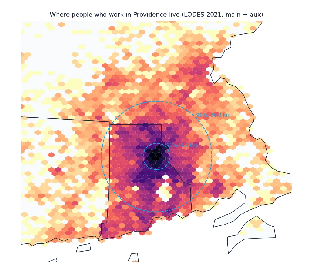
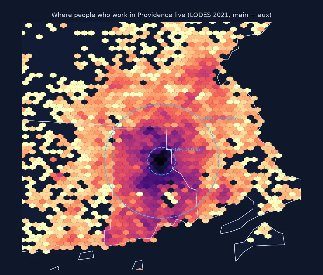
A flow map shows where people go. A catchment map turns it around: for one destination, where do the people come from, and how far? For a city centre, a hospital or a large employer, that is the question behind transit planning, parking demand and recruitment. The answer is a distribution of distances, a distance-decay curve. Two radii summarise it: half the workers live within one, nine in ten within the other. Getting it right for a city near a state line means remembering that the state's main commuting file stops at the border.

This page maps where the people who work in Providence, Rhode Island live, from LODES 2021. It adds the out-of-state workers from the aux file and measures how the catchment changes when they are included.

Quick answer

Take every block pair whose work block is in Providence, place each home block, and compute distances to the job centre of Providence:

prov = od[od.w_geocode.map(TOWN) == PROVIDENCE]
home = prov.h_geocode.map(XY)
ok = home.notna()
d_km = np.array([np.hypot(x - CX, y - CY) for x, y in home[ok]]) / 1000
jobs = prov.S000[ok].to_numpy()
order = np.argsort(d_km); cum = np.cumsum(jobs[order]) / jobs.sum()
r50, r90 = d_km[order][np.searchsorted(cum, 0.5)], d_km[order][np.searchsorted(cum, 0.9)]
print(f"{prov.S000.sum():,} jobs in Providence; {jobs.sum():,} with a placed home; half live within {r50:.1f} km, 90% within {r90:.1f} km")

107,755 jobs in Providence; 105,799 with a placed home; half live within 8.9 km, 90% within 36.8 km

Hexagon map of southern New England coloured on a log scale by the number of Providence jobs held by residents of each cell: very dense in and around Providence, spreading across Rhode Island and into south-eastern Massachusetts and eastern Connecticut, with dashed circles at 8.9 km containing half the workers and 36.8 km containing 90%. — Homes of people who work in Providence, main and aux files combined. Half live within 8.9 km of the city's job centre, 90% within 36.8 km, and the catchment crosses well into Massachusetts.

Add out-of-state workers, measure the unplaced, fit decay

1. Add the workers from other states

The main file holds jobs where home and work are both in Rhode Island. The aux file holds jobs in Rhode Island held by residents of other states. For a city a few kilometres from the Massachusetts line, the difference matters:

by_state = prov.groupby(prov.h_geocode.str[:2]).S000.sum().rename(STATE_NAME).sort_values(ascending=False)
print(by_state.head(5).to_string())
print(f"out-of-state share of Providence jobs: {1 - by_state['Rhode Island'] / by_state.sum():.0%}")

h_geocode
Rhode Island     90975
Massachusetts    13189
Connecticut       1635
New York           804
New Jersey         310
out-of-state share of Providence jobs: 16%

2. Measure what was left unplaced

Home blocks are placed with each state's crosswalk; this page loads Rhode Island, Massachusetts and Connecticut. Jobs held by residents of more distant states stay unplaced. Count them rather than dropping them silently:

unplaced = prov.loc[~ok, "S000"].sum()
print(f"jobs with a home outside RI, MA and CT: {unplaced:,} ({unplaced / prov.S000.sum():.1%}); "
      f"their states: {', '.join(prov.loc[~ok].h_geocode.str[:2].map(STATE_NAME).value_counts().head(3).index)}")

jobs with a home outside RI, MA and CT: 1,956 (1.8%); their states: New York, New Jersey, New Hampshire

3. Compare the catchment with and without `aux`

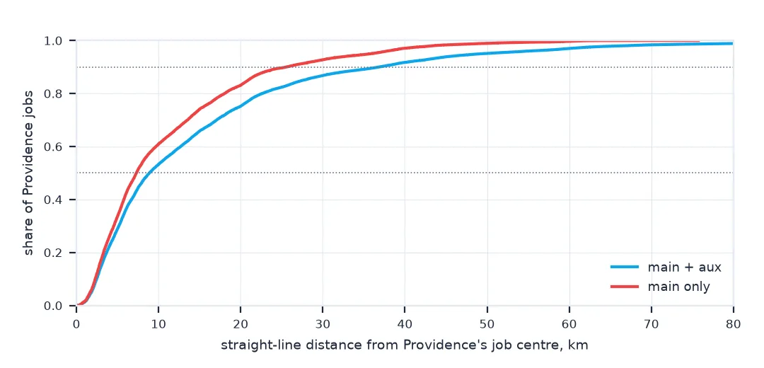
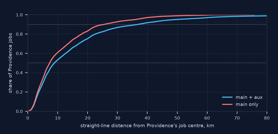
How much does leaving out the other states change the answer?

main_only = prov.h_geocode.str[:2] == "44"
for label, m in (("main only (RI homes)", main_only[ok].to_numpy()), ("main + aux", np.ones(ok.sum(), bool))):
    dd, jj = d_km[m], jobs[m]
    o = np.argsort(dd); c = np.cumsum(jj[o]) / jj.sum()
    print(f"{label:22s}: {jj.sum():>7,} jobs, half within {dd[o][np.searchsorted(c, 0.5)]:.1f} km, "
          f"90% within {dd[o][np.searchsorted(c, 0.9)]:.1f} km")

main only (RI homes)  :  90,975 jobs, half within 7.3 km, 90% within 25.6 km
main + aux            : 105,799 jobs, half within 8.9 km, 90% within 36.8 km

Cumulative distribution of Providence jobs by straight-line distance from the job centre: the main-only curve reaches 50% at 7.3 km and 90% at 25.6 km; with the aux file the curve reaches 50% at 8.9 km and 90% at 36.8 km. — The catchment with and without the out-of-state workers. Leaving out the aux file makes the workforce look more local than it is.

4. Fit the decay

Workers per kilometre band fall off with distance. Fit a straight line to the log of the density of workers per km² against distance; the slope is the decay rate:

bands = np.arange(0, 60, 2)
w, _ = np.histogram(d_km, bands, weights=jobs)
area = np.pi * (bands[1:] ** 2 - bands[:-1] ** 2)
dens = w / area
mid = (bands[1:] + bands[:-1]) / 2
k = (dens > 0) & (mid < 40)
slope, icpt = np.polyfit(mid[k], np.log(dens[k]), 1)
print(f"density of Providence workers falls by {1 - np.exp(slope * 5):.0%} every 5 km (half-distance {np.log(2) / -slope:.1f} km)")

density of Providence workers falls by 52% every 5 km (half-distance 4.7 km)

The closest and farthest workers by town

The data used on this page

LODES version 8, 2021: Rhode Island main and aux OD files for all jobs, and the block crosswalks for Rhode Island, Massachusetts and Connecticut (each block's internal point and town). Distances are in UTM zone 19N (EPSG:32619).

from pathlib import Path

import geopandas as gpd
import matplotlib
matplotlib.use("Agg")
import matplotlib.pyplot as plt
import numpy as np
import pandas as pd
import requests

Path("data").mkdir(exist_ok=True)
L = "https://lehd.ces.census.gov/data/lodes/LODES8/"
SRC = {"ri_od_main_JT00_2021.csv.gz": L + "ri/od/ri_od_main_JT00_2021.csv.gz", "ri_od_aux_JT00_2021.csv.gz": L + "ri/od/ri_od_aux_JT00_2021.csv.gz",
       "ri_xwalk.csv.gz": L + "ri/ri_xwalk.csv.gz", "ma_xwalk.csv.gz": L + "ma/ma_xwalk.csv.gz", "ct_xwalk.csv.gz": L + "ct/ct_xwalk.csv.gz"}
for name, url in SRC.items():
    if not Path("data", name).exists():
        Path("data", name).write_bytes(requests.get(url, timeout=600).content)
dt = {"w_geocode": str, "h_geocode": str}
od = pd.concat([pd.read_csv(f"data/ri_od_{k}_JT00_2021.csv.gz", dtype=dt) for k in ("main", "aux")], ignore_index=True)
xw = pd.concat([pd.read_csv(f"data/{s}_xwalk.csv.gz", dtype=str, usecols=["tabblk2020", "ctycsub", "blklatdd", "blklondd"])
                for s in ("ri", "ma", "ct")]).set_index("tabblk2020")
pts = gpd.GeoSeries(gpd.points_from_xy(xw.blklondd.astype(float), xw.blklatdd.astype(float)), index=xw.index, crs=4326).to_crs(32619)
XY = pd.Series(list(zip(pts.x, pts.y)), index=xw.index)
TOWN = xw.ctycsub
PROVIDENCE = "4400759000"                                                    # Providence city, county subdivision GEOID
wj = od[od.w_geocode.map(TOWN) == PROVIDENCE].groupby("w_geocode").S000.sum()
CX = np.average([XY[b][0] for b in wj.index], weights=wj); CY = np.average([XY[b][1] for b in wj.index], weights=wj)
STATE_NAME = {"44": "Rhode Island", "25": "Massachusetts", "09": "Connecticut", "36": "New York", "34": "New Jersey",
              "33": "New Hampshire", "23": "Maine", "42": "Pennsylvania", "51": "Virginia", "50": "Vermont", "12": "Florida"}
print(f"{len(od):,} block pairs (main + aux); {len(xw):,} blocks placed in RI, MA and CT")

426,844 block pairs (main + aux); 182,853 blocks placed in RI, MA and CT

Example 1: the closest and farthest workers by town

towns = prov[ok].assign(km=d_km, town=prov.loc[ok, "h_geocode"].map(TOWN)).groupby("town").agg(jobs=("S000", "sum"), km=("km", "median"))
print(f"{len(towns)} home towns; median distance of towns sending 500+ workers: "
      f"{towns[towns.jobs >= 500].km.median():.1f} km, farthest of those {towns[towns.jobs >= 500].km.max():.1f} km")

461 home towns; median distance of towns sending 500+ workers: 16.6 km, farthest of those 60.1 km

A catchment is one destination read as a distribution

A catchment is a flow table filtered to one destination and read as a distribution. Its shape is the distance-decay curve: many workers close by, fewer and fewer farther out. Most of the information is in two radii and one rate. Half of Providence's workers live within the first radius, nine in ten within the second, and the decay rate says how fast density falls between them. Those numbers transfer between places in a way that a map does not.

Where Providence's workers live, by state.

The aux file is the easy thing to miss, and here it changes the answer: 16% of Providence's jobs are held by people from other states, and the 90% radius grows from 25.6 km to 36.8 km once they are included. Providence sits a few kilometres from the Massachusetts line, and many of its workers live on the other side. A catchment built from the main file alone stops at the state border by construction, and it understates both the size of the workforce and how far it travels. Any destination near a state boundary has the same problem.

Placing homes, straight lines and job centres

Catchment problems and fixes.

Placing homes needs each home state's crosswalk; load the states that matter and report the jobs left unplaced.
Straight-line distance understates travel distance; route a sample on the street network for a correction factor.
Jobs, not people: LODES counts jobs; a worker with two Providence jobs counts twice.
Job centre: the job-weighted centre of Providence is used as the origin of distances, not the city's polygon centroid.
Density bands far out contain few workers and noisy densities; fit the decay over the inner bands only.

Internal links

How to map commuting flows from LODES — the town-to-town flows
How to build desire lines — the same data as lines

FAQ

What is a commuting catchment?

The area from which a destination's workers come, usually summarised by the distances within which half and nine tenths of them live.

What is distance decay?

The fall in the number (or density) of trips as distance from the destination increases, often close to exponential over the inner range.

Why do I need the LODES aux file?

The main file covers only jobs where home and work are in the same state; aux adds jobs held by residents of other states, which matters near state borders.

How do I measure catchment radius in Python?

Sort the home distances, take the cumulative sum of jobs, and read off the distance where the cumulative share reaches 50% or 90%.