
How to Read County-to-County Migration Flows in Python
On this page
Problem statement
The US Census Bureau publishes how many people moved between every pair of US counties, from the American Community Survey. It is the most detailed open origin–destination dataset in the country, and the raw material for flow maps and migration analysis. It also arrives as a workbook built for reading, not for code. There is one sheet per state and four header rows above the data. Footnotes sit below it. Codes must keep their leading zeros, and some rows are foreign regions. Every estimate carries a margin of error, and for most county pairs that margin is as large as the estimate itself.
This page reads the 2016–2020 flows for Los Angeles County into a tidy table. It checks the totals and separates the flows that can be trusted from the ones that cannot.
Quick answer
Read one state's sheet with explicit column names, skip the header rows, keep codes as strings, and drop the footnote rows:
COLS = ["a_st", "a_cty", "b_st", "b_cty", "a_state", "a_county", "b_state", "b_county",
        "flow", "flow_moe", "counter", "counter_moe", "net", "net_moe", "gross", "gross_moe"]
ca = pd.read_excel(XLSX, sheet_name="California", header=None, skiprows=3, names=COLS, dtype=str)
ca = ca[ca.a_cty.notna()]                                              # footnotes have no county code
for c in COLS[8:]:
    ca[c] = pd.to_numeric(ca[c], errors="coerce")
la = ca[ca.a_cty == "037"].copy()                                       # Los Angeles County
print(f"{len(ca):,} California rows; Los Angeles County: {len(la):,} partner geographies")
16,490 California rows; Los Angeles County: 1,243 partner geographies
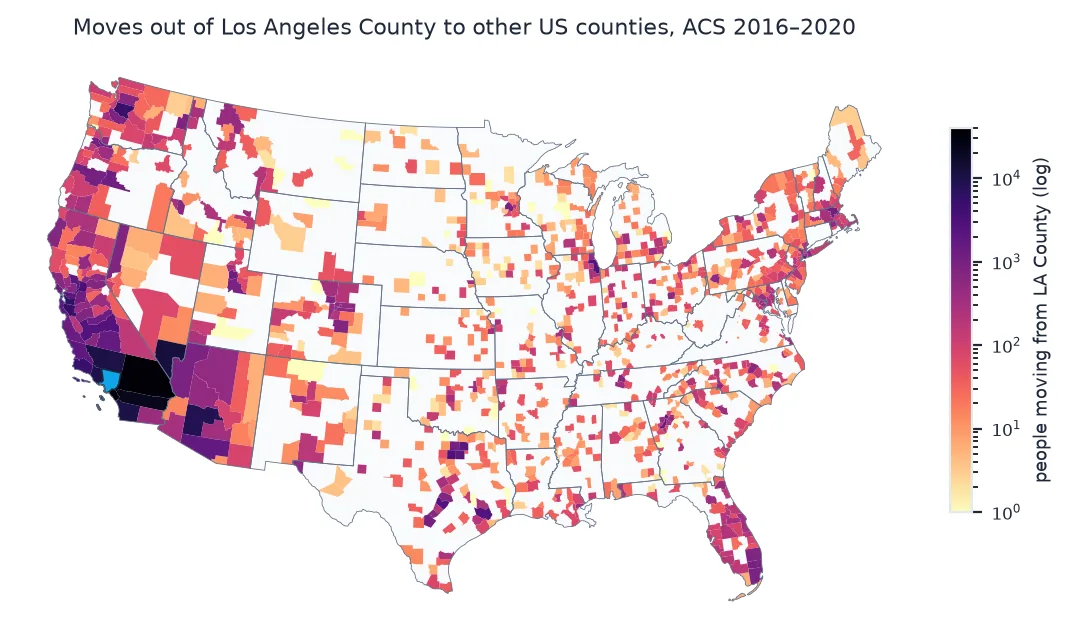
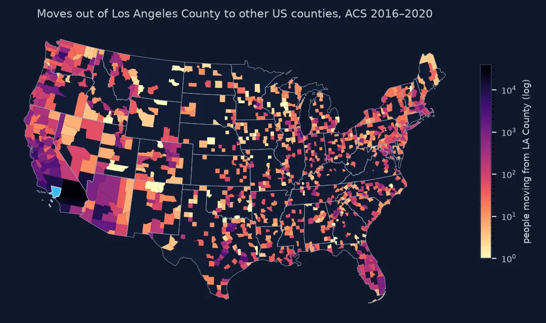
Column directions, foreign regions, margins of error
1. Know which way each column points
Each row pairs a county A (the sheet's state) with a geography B. flow is people who moved from B to A; counter is people who moved from A to B; net = flow − counter; gross = flow + counter. Read them back as in and out of Los Angeles County:
us = la[la.b_st.str.fullmatch(r"\d{3}")]                                # US states, not foreign regions
print(f"into LA from other US counties: {us.flow.sum():,.0f}; out of LA to other US counties: {us.counter.sum():,.0f}; "
      f"net {us.net.sum():+,.0f}")
print(us.nlargest(5, "counter")[["b_county", "b_state", "counter", "flow", "net"]].to_string(index=False))
into LA from other US counties: 201,675; out of LA to other US counties: 325,093; net -123,418
b_county b_state counter flow net
Orange County California 38761.0 23839 -14922.0
San Bernardino County California 34920.0 15590 -19330.0
Riverside County California 23292.0 10232 -13060.0
Clark County Nevada 12873.0 3349 -9524.0
Kern County California 10503.0 5058 -5445.0
2. Separate foreign regions
Rows whose B code is letters, such as ASI or EUR, are moves from abroad. The ACS cannot see people who left the country, so these rows have a flow into A but no counterflow:
abroad = la[~la.b_st.str.fullmatch(r"\d{3}")]
print(abroad[["b_st", "b_state", "flow", "counter"]].to_string(index=False))
print(f"moved to LA from abroad: {abroad.flow.sum():,.0f}")
b_st b_state flow counter
AFR Africa 2278 NaN
ASI Asia 33605 NaN
CAM Central America 12745 NaN
CAR Caribbean 1006 NaN
EUR Europe 8855 NaN
ISL U.S. Island Areas 321 NaN
NAM Northern America 1410 NaN
OCE Oceania and At Sea 1397 NaN
SAM South America 4226 NaN
moved to LA from abroad: 65,843
3. Judge each estimate by its margin of error
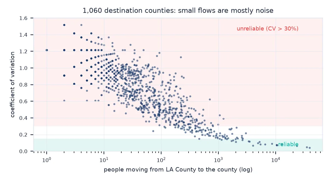
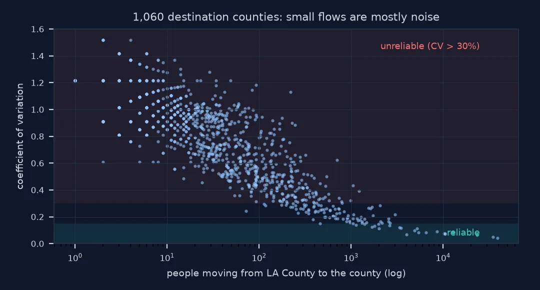
The margins are 90% confidence intervals. Convert them to a coefficient of variation (CV = MOE / 1.645 / estimate) and sort the flows by reliability:
us = us.assign(cv=us.counter_moe / 1.645 / us.counter)
bands = pd.cut(us.cv, [0, 0.15, 0.30, np.inf], labels=["reliable (CV < 15%)", "use with care", "unreliable (CV > 30%)"])
summary = us.groupby(bands, observed=False).agg(pairs=("counter", "size"), movers=("counter", "sum"))
summary["share of movers"] = summary.movers / summary.movers.sum()
print(summary.to_string(float_format=lambda v: f"{v:.1%}" if v < 1 else f"{v:,.0f}"))
pairs movers share of movers
cv
reliable (CV < 15%) 23 195,505 60.1%
use with care 79 65,494 20.1%
unreliable (CV > 30%) 958 64,094 19.7%
4. Check the totals
A flow table should add up. The workbook's own gross column is flow plus counterflow, and net is their difference; check both:
both = us.dropna(subset=["flow", "counter"])
print("gross = flow + counter on every row:", bool(((both.flow + both.counter) == both.gross).all()))
print("net = flow - counter on every row:  ", bool(((both.flow - both.counter) == both.net).all()))
gross = flow + counter on every row: True
net = flow - counter on every row: True
A long table of county flows for mapping
The data used on this page
County-to-county migration flows, 2016–2020 ACS 5-year estimates from the US Census Bureau (the "ins, outs, nets, gross" workbook), and county outlines from the cartographic boundary files, 2023.
from pathlib import Path

import geopandas as gpd
import numpy as np
import pandas as pd
import requests

Path("data").mkdir(exist_ok=True)
XLSX = Path("data/county-to-county-2016-2020-ins-outs-nets-gross.xlsx")
if not XLSX.exists():
    XLSX.write_bytes(requests.get("https://www2.census.gov/programs-surveys/demo/tables/geographic-mobility/2020/"
                                  "county-to-county-migration-2016-2020/county-to-county-migration-flows/" + XLSX.name, timeout=600).content)
if not Path("data/cb_2023_us_county_20m.zip").exists():
    Path("data/cb_2023_us_county_20m.zip").write_bytes(requests.get("https://www2.census.gov/geo/tiger/GENZ2023/shp/cb_2023_us_county_20m.zip", timeout=300).content)
counties = gpd.read_file("data/cb_2023_us_county_20m.zip")
print(f"workbook {XLSX.stat().st_size / 1e6:.1f} MB; {len(counties):,} county outlines")
workbook 30.4 MB; 3,222 county outlines
Example 1: a long table for mapping
long = us.assign(dest=us.b_st.str[1:] + us.b_cty, movers=us.counter)[["dest", "b_county", "b_state", "movers", "counter_moe", "cv"]]
mapped = counties.merge(long, left_on="GEOID", right_on="dest", how="inner")
print(f"{len(mapped):,} of {len(long):,} destination counties matched an outline; "
      f"unmatched: {sorted(set(long.dest) - set(counties.GEOID))[:5]}")
1,226 of 1,234 destination counties matched an outline; unmatched: ['09001', '09003', '09005', '09007', '09009']
A matrix stored as a list
A migration flow table is a matrix stored as a list. Each row answers "how many people moved between these two places, in which direction", with an uncertainty attached. The workbook stores each county pair from both sides, once in each state's sheet. Reading it is mostly about orientation: which column is in and which is out, which rows are real places, which codes are text.
The margins of error are the part most analyses skip and most need. The ACS is a sample. A flow of a few dozen people between two counties rests on a handful of survey responses, and its 90% interval often runs from zero to double the estimate. The big flows, such as Los Angeles to its neighbouring counties, are solid. The long tail of small flows is mostly noise, and most of it sits there by count, not by people.
State code widths, Connecticut and Puerto Rico
- State code width: B codes are three characters (
006); county GEOIDs are two-digit state plus three-digit county (06059). Drop the leading zero of the B state code before joining. - Connecticut replaced counties with planning regions in 2022; 2016–2020 flows use the old counties, which the 2023 outlines no longer contain.
- Blank counterflows mean "not available", not zero; keep them as missing.
- Puerto Rico has its own sheet; foreign moves out of the US are not measured at all.
- Five-year estimates describe 2016–2020 as a whole, not any single year.
Internal links
- How to make a flow map in Python — drawing these flows
- Gross vs net migration explained — why net hides most moves
FAQ
Where can I download county-to-county migration data?
From the Census Bureau's geographic mobility tables: the 2016–2020 ACS county-to-county migration flows, as workbooks or a fixed-width text file.
What is the difference between flow and counterflow?
In this workbook, flow is moves from geography B into county A; counterflow is moves from county A to B.
How reliable are county migration flows?
Large flows are reliable; most small ones are not. Convert the 90% margin of error to a coefficient of variation and treat CVs above 30% with suspicion.
Why do my county codes not match the map?
Codes lost their leading zeros, or the B state code still has its three-digit form. Read codes as strings and build five-digit GEOIDs.