
How to delineate field boundaries from imagery in Python
Problem statement
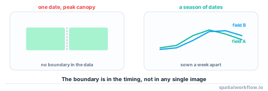
Where no agricultural parcel register exists, the boundaries have to come from the imagery — and a single date cannot provide them, because two adjacent fields growing the same crop at the same stage are the same colour.
What separates fields is time. Two fields differ because they were sown on different dates, with different varieties, and harvested in different weeks. A stack of dates turns an invisible boundary into a sharp one, and the delineation becomes a segmentation of a multi-band image whose bands are dates.
This guide builds that stack from real Sentinel-2 data, segments it, and checks the result against the artefacts that always appear.
Quick answer
Segment a temporal stack, not a single image:
import numpy as np
from skimage.segmentation import felzenszwalb
from skimage.filters import sobel

stack = np.dstack([ndvi_date for ndvi_date in dates])       # rows × cols × dates
stack = np.nan_to_num(stack, nan=float(np.nanmedian(stack)))

segments = felzenszwalb(stack, scale=200, sigma=1.0, min_size=250, channel_axis=2)
print(f"{segments.max() + 1:,} segments from {stack.shape[2]} dates")
scale controls how large the segments are and is the parameter to sweep. min_size is in pixels — at 20 m resolution, 250 pixels is 10 ha, which is a sensible floor for arable land and far too large for horticulture.
Step-by-step solution
1. Build a clean temporal stack
Cloud-screened, gap-filled and on a common grid. Twenty dates across a season is plenty; the reference series had 21 dates from 7 March to 6 September with 19 of them more than 60% clear.
2. Use an index that does not saturate
The stack's job is to separate fields, and NDVI is flat across the whole of mid-summer — on the reference scene, 55.9% of vegetation pixels were above 0.8. A red-edge index keeps its dynamic range and therefore keeps the boundaries.
3. Reduce the dates to a small number of components
Twenty correlated bands is more than any segmenter needs. A principal component transform reduces them to three or four that hold nearly all the variance, which is faster and less noisy.
4. Segment
Felzenszwalb, SLIC and watershed on a gradient all work. Felzenszwalb needs the least tuning and produces variable-sized segments, which suits fields. SLIC produces roughly equal-sized superpixels, which does not.
5. Merge segments that are the same field
Over-segmentation is easier to fix than under-segmentation. Merging adjacent segments whose temporal profiles are close recovers fields that were split by a tramline or a wet patch.
6. Filter the artefacts
Slivers, ribbons along roads and hedges, and segments that are mostly non-agricultural. Area and compactness catch most of them — a reference OSM layer of the same area had 3.7% of parcels under half a hectare and 9.1% with compactness below 0.3, which is roughly what a good delineation should also produce.
7. Validate against something
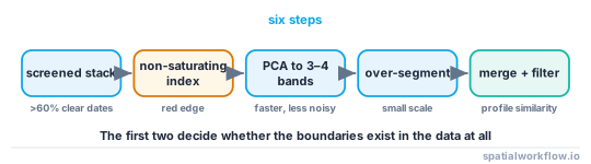
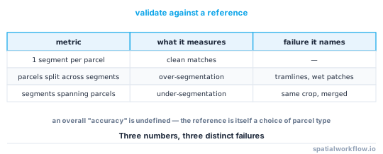
Where any reference parcels exist — a register, a sample of hand-digitised fields, OSM — compare. The useful metrics are the fraction of reference parcels matched by one segment, the fraction split across several, and the fraction of segments that span two reference parcels.
Code examples
Example 1 — build the stack from a STAC search
import json, urllib.request, os, numpy as np, rasterio
from rasterio.warp import transform_bounds
from rasterio.windows import from_bounds

os.environ.setdefault("GDAL_DISABLE_READDIR_ON_OPEN", "EMPTY_DIR")
os.environ.setdefault("AWS_NO_SIGN_REQUEST", "YES")
SCALE = 1e-4

def search(bbox, start, end, cloud=20, limit=60):
    body = {"collections": ["sentinel-2-l2a"], "bbox": bbox,
            "datetime": f"{start}/{end}", "limit": limit,
            "query": {"eo:cloud_cover": {"lt": cloud}}}
    req = urllib.request.Request("https://earth-search.aws.element84.com/v1/search",
        data=json.dumps(body).encode(), headers={"Content-Type": "application/json"})
    with urllib.request.urlopen(req, timeout=120) as r:
        return json.loads(r.read())["features"]

def window_read(href, bbox, step=1):
    with rasterio.open(href) as src:
        b = transform_bounds("EPSG:4326", src.crs, *bbox)
        win = from_bounds(*b, transform=src.transform)
        return (src.read(1, window=win).astype("float32")[::step, ::step],
                src.crs, src.window_transform(win))

def build_stack(bbox, start, end, min_clear=0.6):
    feats = sorted(search(bbox, start, end), key=lambda f: f["properties"]["datetime"])
    layers, dates = [], []
    for f in feats:
        a = f["assets"]
        nir, crs, tr = window_read(a["nir"]["href"], bbox, 2)
        re1, _, tr20 = window_read(a["rededge1"]["href"], bbox, 1)
        scl, _, _ = window_read(a["scl"]["href"], bbox, 1)
        h = min(nir.shape[0], re1.shape[0], scl.shape[0])
        w = min(nir.shape[1], re1.shape[1], scl.shape[1])
        nir, re1, scl = nir[:h, :w] * SCALE, re1[:h, :w] * SCALE, scl[:h, :w]
        clear = np.isin(scl, [4, 5, 6])
        if clear.mean() < min_clear:
            continue
        with np.errstate(invalid="ignore", divide="ignore"):
            ndre = np.where(clear, (nir - re1) / (nir + re1), np.nan)
        layers.append(ndre)
        dates.append(f["properties"]["datetime"][:10])
    return np.dstack(layers), dates, crs, tr20
Dropping dates below 60% clear is a decision worth reporting: on the reference series that removed 2 of 21 dates.
Example 2 — reduce, segment and vectorise
import numpy as np, geopandas as gpd
from sklearn.decomposition import PCA
from skimage.segmentation import felzenszwalb
from rasterio.features import shapes
from shapely.geometry import shape

def delineate(stack, transform, crs, n_components=4, scale=200, min_size=250):
    h, w, t = stack.shape
    flat = stack.reshape(-1, t)
    med = np.nanmedian(flat, axis=0)
    flat = np.where(np.isfinite(flat), flat, med)

    pca = PCA(n_components=min(n_components, t)).fit(flat)
    comp = pca.transform(flat).reshape(h, w, -1)
    print("explained variance:", np.round(pca.explained_variance_ratio_, 3))

    comp = (comp - comp.min(axis=(0, 1))) / np.ptp(comp, axis=(0, 1))
    seg = felzenszwalb(comp, scale=scale, sigma=1.0, min_size=min_size,
                       channel_axis=2)

    polys = [{"seg": int(v), "geometry": shape(g)}
             for g, v in shapes(seg.astype("int32"), transform=transform)]
    g = gpd.GeoDataFrame(polys, crs=crs).dissolve("seg", as_index=False)
    g["area_ha"] = g.area / 1e4
    g["compactness"] = 4 * np.pi * g.area / (g.length ** 2)
    print(f"{len(g):,} segments; median {g.area_ha.median():.1f} ha, "
          f"{(g.area_ha < 0.5).sum()} under 0.5 ha, "
          f"{(g.compactness < 0.3).sum()} with compactness below 0.3")
    return g, seg
Example 3 — merge over-segmented neighbours
import numpy as np, geopandas as gpd
from scipy import ndimage

def merge_similar(seg, stack, threshold=0.05):
    """Merge adjacent segments whose mean temporal profiles are close."""
    n = seg.max() + 1
    profiles = np.stack([
        np.nanmean(stack[seg == i], axis=0) if (seg == i).any() else np.zeros(stack.shape[2])
        for i in range(n)])

    parent = np.arange(n)
    def find(a):
        while parent[a] != a:
            parent[a] = parent[parent[a]]
            a = parent[a]
        return a

    # adjacency from a one-pixel dilation of each label boundary
    right = np.c_[seg[:, :-1].ravel(), seg[:, 1:].ravel()]
    down = np.c_[seg[:-1, :].ravel(), seg[1:, :].ravel()]
    pairs = np.unique(np.vstack([right, down]), axis=0)
    pairs = pairs[pairs[:, 0] != pairs[:, 1]]

    for a, b in pairs:
        d = np.nanmean(np.abs(profiles[a] - profiles[b]))
        if d < threshold:
            ra, rb = find(a), find(b)
            if ra != rb:
                parent[ra] = rb

    merged = np.vectorize(find)(seg)
    print(f"{n:,} segments → {len(np.unique(merged)):,} after merging at {threshold}")
    return merged
Merging on the mean absolute difference between temporal profiles is crude and effective. The threshold is the parameter to sweep, and the right value depends on the index's dynamic range — which is another reason to use one that does not saturate.
Explanation
Why a single date cannot work
Field boundaries are management boundaries, and management is only visible when it differs. Two neighbouring fields of winter wheat sown a week apart are indistinguishable at peak canopy and clearly different at emergence and at senescence. A single image samples one moment and therefore finds only the boundaries that happen to be expressed then.
Why the index choice is not cosmetic here
A saturated index has no dynamic range, so adjacent fields that differ by real biomass have the same value and no boundary appears. Between 12 and 30 June the reference series held NDVI at 0.770–0.776 — three weeks in which NDVI would have contributed nothing to a segmentation, while NDRE varied over 0.264 across fields in the same period.
Why over-segmentation is the safer failure
A field split into three segments can be merged with a rule. Three fields merged into one segment cannot be separated without going back to the imagery, and any statistic computed on it is a weighted average of three different crops. Tune towards smaller segments and merge.
Why to validate on match fractions rather than on an overall accuracy
"Accuracy" for a delineation is ill-defined, because the reference itself is a choice of parcel type. The useful numbers are how many reference parcels are covered by exactly one segment, how many are split, and how many segments straddle two parcels. Those three name the failure modes directly.
Edge cases or notes
- Tramlines split a field in the segmentation; merging fixes it.
- Grassland has no strong seasonal signal and delineates poorly.
- Irrigation circles are easy, hedges are hard.
- Mixed cropping within a field produces genuine internal boundaries.
- The stack must be on one grid. Reproject before stacking, not after.
- Gap-fill before PCA. NaNs propagate through the decomposition.
min_sizeis in pixels. Convert to hectares before choosing it.- Record the dates used. A delineation is a statement about a season.
Internal links
- Field boundary data explained: where it comes from — whether you need to delineate at all
- Delineated field boundaries merge fields or swallow roads — the failure modes
- Vegetation indices explained: NDVI, EVI, NDRE and when each fails — why the index matters here
- How to classify crop types from a satellite time series — the next step
- How to classify land cover in Python — the pixel-based alternative
- How to convert raster to vector in Python — vectorising the segments
- How to build a STAC-based data cube with xarray — assembling the stack
- How to mask clouds in Sentinel-2 imagery in Python — screening the dates
FAQ
Can I delineate fields from a single image?
No. Adjacent fields with the same crop at the same stage are the same colour. Boundaries appear across a season, not within one date.
Which index should I stack?
One that does not saturate — a red-edge index. NDVI is flat across most of mid-summer, which is a large part of the season contributing nothing.
How many dates do I need?
Fifteen to twenty across a season is ample, provided they span emergence and senescence as well as the peak.
Which segmentation algorithm?
Felzenszwalb needs the least tuning and produces variable-sized segments, which suits fields. SLIC's equal-sized superpixels do not.
Should I aim for over- or under-segmentation?
Over. Merging adjacent segments with similar temporal profiles is a rule; separating merged fields is not.
How do I know if it worked?
Compare with any reference parcels you have, and report three numbers: parcels matched by one segment, parcels split across several, and segments spanning two parcels.