
Delineated field boundaries merge fields or swallow roads
Problem statement
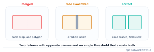
The segmentation ran, the polygons look plausible, and two things are wrong. Some adjacent fields with the same crop have become one polygon, and some polygons include the road, the ditch and the hedge between two fields.
Both are the same mechanism from opposite directions: the segmenter grouped pixels whose temporal profiles were similar enough, and "similar enough" is one parameter. Tighten it and fields split into tramline-sized fragments; loosen it and neighbouring wheat fields merge. There is no setting that does both, which is why the fix is in the features and the post-processing rather than in the threshold.
Quick answer
Diagnose by measuring what the segments contain, not by looking at them:
import numpy as np, geopandas as gpd

seg["area_ha"] = seg.area / 1e4
seg["compactness"] = 4 * np.pi * seg.area / (seg.length ** 2)

print(f"{len(seg):,} segments; median {seg.area_ha.median():.1f} ha, "
      f"max {seg.area_ha.max():.1f} ha")
print(f"over 3x the median area: {(seg.area_ha > 3 * seg.area_ha.median()).sum()} "
      "(candidate merges)")
print(f"compactness below 0.3: {(seg.compactness < 0.3).sum()} "
      "(candidate ribbons along roads)")
A reference OpenStreetMap layer for the same Dutch polder area had a median parcel of 24.74 ha, a maximum of 193.3 ha, 3.7% under half a hectare and 9.1% with a compactness below 0.3. A delineation that produces a very different profile is describing something other than fields.
Step-by-step solution
1. Check whether the boundary exists in the data at all
Two fields of the same crop, sown the same week, differ only slightly. Plot the temporal profiles of the two halves of a merged segment: if they are indistinguishable, no segmenter can separate them and the fix is more dates, a different index, or an external boundary source.
2. Check the index for saturation
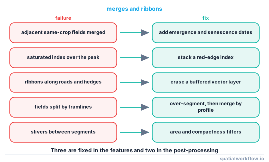
A saturated index has no dynamic range, so real differences disappear. On the reference scene, 55.9% of vegetation pixels were above NDVI 0.8, and the field-median NDVI sat between 0.770 and 0.776 for eighteen days — three weeks contributing nothing to the segmentation. A red-edge index keeps its range.
3. Add the dates that separate fields
Emergence and senescence separate fields far better than peak canopy does, because sowing and harvest dates differ even when the crop does not. If the stack is peak-heavy, the merges are inevitable.
4. Over-segment deliberately, then merge
Set the segmentation scale small enough that fields split, then merge adjacent segments whose profiles are close. Merging is a rule you control; separating merged fields is not.
5. Cut the linear features out rather than tuning them away
Roads, hedges and ditches are in OpenStreetMap. Buffering them and erasing them from the segments removes the ribbons without touching the threshold.
6. Use an edge signal as well as a region signal
Segmenters that use only region similarity have no reason to place a boundary at a hedge. Adding a gradient layer — the temporal standard deviation, or the magnitude of the gradient of the first principal component — gives the segmenter an edge to snap to.
7. Filter the artefacts by shape
Ribbons have low compactness, slivers have small area, and segments that span two fields are unusually large. All three are one line each.
Code examples
Example 1 — test whether a merged segment really is two fields
import numpy as np
from sklearn.cluster import KMeans

def split_test(stack, seg, seg_id, min_pixels=200):
    """Cluster the temporal profiles inside one segment into two."""
    mask = seg == seg_id
    if mask.sum() < min_pixels:
        return None
    X = stack[mask]
    ok = np.isfinite(X).all(axis=1)
    if ok.sum() < min_pixels:
        return None

    km = KMeans(n_clusters=2, n_init=10, random_state=0).fit(X[ok])
    a, b = X[ok][km.labels_ == 0], X[ok][km.labels_ == 1]
    sep = np.abs(a.mean(axis=0) - b.mean(axis=0))
    pooled = np.sqrt((a.var(axis=0) + b.var(axis=0)) / 2)
    effect = float(np.nanmax(sep / np.where(pooled == 0, np.nan, pooled)))

    return {"pixels": int(ok.sum()),
            "balance": round(float(min(len(a), len(b)) / ok.sum()), 3),
            "max_effect_size": round(effect, 2),
            "verdict": "two fields" if effect > 1.5 and min(len(a), len(b)) / ok.sum() > 0.2
                       else "one field"}
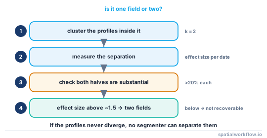
An effect size above about 1.5 on at least one date, with both halves substantial, means the segment contains two genuinely different profiles. Below that, the merge is not recoverable from these data.
Example 2 — erase linear features
import geopandas as gpd

def erase_linear(seg, roads, hedges=None, buffer_m=4, min_area_ha=0.5):
    lines = [roads] + ([hedges] if hedges is not None else [])
    mask = gpd.GeoDataFrame(
        geometry=[g.buffer(buffer_m) for gdf in lines for g in gdf.geometry],
        crs=seg.crs).dissolve()

    out = gpd.overlay(seg, mask, how="difference").explode(index_parts=False)
    out["area_ha"] = out.area / 1e4
    dropped = out[out.area_ha < min_area_ha]
    if len(dropped):
        print(f"erasing linear features split off {len(dropped)} fragments "
              f"({dropped.area_ha.sum():.2f} ha)")
    return out[out.area_ha >= min_area_ha]
Buffering by half the road width plus the pixel size is about right. Too small and the ribbon survives; too large and it eats the headland.
Example 3 — profile the result against a reference
import numpy as np, geopandas as gpd, pandas as pd

def compare_profile(seg, reference, crs=28992):
    rows = []
    for name, g in (("delineated", seg), ("reference", reference)):
        g = g.to_crs(crs)
        a = g.area / 1e4
        c = 4 * np.pi * g.area / (g.length ** 2)
        rows.append({"layer": name, "n": len(g),
                     "median_ha": round(float(a.median()), 2),
                     "max_ha": round(float(a.max()), 1),
                     "under_0.5_ha": int((a < 0.5).sum()),
                     "compact_below_0.3": int((c < 0.3).sum()),
                     "total_ha": round(float(a.sum()))})
    df = pd.DataFrame(rows)
    print(df.to_string(index=False))
    return df
Comparing the shape profile with a reference layer of the same area catches both failure modes at once: merges push the median and maximum area up, ribbons push the low-compactness count up.
Explanation
Why the same parameter causes both failures
A region-merging segmenter groups adjacent pixels whose values differ by less than a threshold. The distance between two fields of different crops is large; between two fields of the same crop it is small; between a field and the tramline running through it, smaller still. Those three distances are not separated by any single threshold, so one setting always merges something that should be split or splits something that should be merged.
Why more dates help and a better algorithm does not
Two fields of the same crop differ in when they were sown and when they were harvested, which is expressed at emergence and senescence and almost nowhere else. A stack that samples those periods contains the boundary; one that samples only the peak does not, and no segmenter can find information that is not there.
Why linear features should be erased rather than segmented around
A hedge or a road is three to eight metres wide, which at 10–20 m resolution is a partial pixel with a mixed spectral signature that resembles neither field. Asking a segmenter to place a boundary on such a pixel is asking for trouble; erasing a known vector layer is deterministic, reversible and uses information the imagery does not contain.
Why over-segmentation is the safe direction
A merged segment has lost information irretrievably: the mean profile of two fields is not either field, and every statistic computed on it is a weighted average of two crops. A split field retains all of it, and merging adjacent segments by profile similarity is a rule with a parameter you can sweep and validate.
Edge cases or notes
- Tramlines split fields at fine scales; merging recovers them.
- A field with two crops genuinely has an internal boundary.
- Grassland has little seasonal signal and delineates poorly whatever you do.
- Irrigation circles are easy; small irregular fields are not.
min_sizeis in pixels. Convert to hectares before setting it.- Erasing roads splits a field in two where a track crosses it; merge afterwards.
- Compare the shape profile with a reference rather than judging by eye.
- Record the dates used. A delineation is a statement about one season.
Internal links
- How to delineate field boundaries from imagery in Python — the pipeline this fixes
- Field boundary data explained: where it comes from — whether to delineate at all
- Vegetation indices explained: NDVI, EVI, NDRE and when each fails — why saturation causes merges
- NDVI stops responding in a dense canopy — the flat peak
- How to simplify geometry in GeoPandas — cleaning the polygons
- How to fix gaps and overlaps in a polygon coverage — after erasing
- How to download OpenStreetMap data in Python — getting the roads and hedges
- How to convert raster to vector in Python — the vectorisation step
FAQ
Why did two fields merge into one polygon?
Because their temporal profiles were too similar for the threshold — usually the same crop sown at the same time, or a stack dominated by saturated peak-season dates.
Why does my polygon include the road?
Because a road pixel at 10–20 m resolution is a mixed pixel that resembles neither field. Erase a buffered road layer rather than trying to tune it away.
Can I just change the segmentation threshold?
No. The same parameter controls both failures in opposite directions. Over-segment and merge instead.
How do I know whether a merged segment is really two fields?
Cluster the temporal profiles inside it into two and measure the separation. An effect size above about 1.5 on at least one date with both halves substantial means two fields.
Which dates matter most?
Emergence and senescence. Sowing and harvest dates differ between fields even when the crop does not; peak canopy does not separate them.
How do I check the result?
Compare the area and compactness profile with a reference layer for the same area. Merges raise the median area; ribbons raise the low-compactness count.