
How to build management zones with clustering in Python
Problem statement
Clustering a field into zones is four lines of scikit-learn and a great many decisions: which layers, how to normalise them, how many clusters, how to smooth the result, and how to tell whether the zones mean anything.
The failure is always the same shape — zones that look convincing, follow the previous year's weather, and explain almost none of the variation in any other year. The fix is not a better algorithm; it is stable inputs, a held-out year and a test that produces a number.
This guide builds the zoning, smooths it into something a machine can drive, and evaluates it.
Quick answer
import numpy as np
from sklearn.cluster import KMeans
from sklearn.preprocessing import StandardScaler

X = np.column_stack([mean_z.ravel(), stability.ravel(), elevation.ravel()])
ok = np.isfinite(X).all(axis=1)

labels = np.full(X.shape[0], -1, dtype="int16")
km = KMeans(n_clusters=3, n_init=20, random_state=0).fit(StandardScaler().fit_transform(X[ok]))
labels[ok] = km.labels_

# order zones by productivity so the labels mean the same thing every run
order = np.argsort([mean_z.ravel()[labels == k].mean() for k in range(3)])
labels[ok] = np.vectorize({old: new for new, old in enumerate(order)}.get)(labels[ok])
zones = labels.reshape(mean_z.shape)
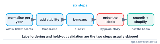
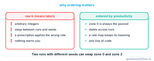
Re-ordering the labels by productivity is not cosmetic. K-means labels are arbitrary, so without it zone 1 means something different every time the script runs, and a prescription written against last week's run applies the wrong rates.
Step-by-step solution
1. Assemble layers that do not change between years
A multi-year vegetation index mean, its temporal standard deviation, elevation and its derivatives, and soil electrical conductivity if a survey exists. Put every year on a common grid first.
2. Normalise each year within the field before combining
Absolute levels differ between seasons. A within-field z-score per year removes the season and keeps the pattern, which is the thing the zones are for.
3. Include stability as its own variable
The temporal standard deviation separates a consistently mediocre area from an alternately excellent and terrible one, which a mean cannot.
4. Choose the number of clusters, and justify it
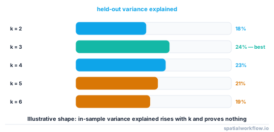
Sweep two to six and look at the silhouette score, the variance explained in a held-out year, and whether the smallest zone is large enough to manage. Two or three usually wins on all three.
5. Order the labels and smooth the result
A modal filter removes speckle, a minimum area removes unmanageable fragments, and simplifying at roughly half the implement width removes detail the machine cannot follow.
6. Validate on a year that was not used
Fit the zones on some years, compute the variance explained in another. That number is the zoning's value, and it is usually much lower than the within-sample figure.
7. Publish the inputs with the zones
Which years, which layers, which parameters. A zone map without them cannot be reproduced or updated.
Code examples
Example 1 — stack, normalise and cluster
import numpy as np
from sklearn.cluster import KMeans
from sklearn.preprocessing import StandardScaler
from sklearn.metrics import silhouette_score

def build_inputs(year_arrays: dict, extra: dict = None):
    z = {}
    for label, a in year_arrays.items():
        a = np.asarray(a, dtype="float32")
        z[label] = (a - np.nanmean(a)) / np.nanstd(a)
    zs = np.stack(list(z.values()))
    out = {"mean_z": np.nanmean(zs, axis=0), "stability": -np.nanstd(zs, axis=0)}
    for k, v in (extra or {}).items():
        v = np.asarray(v, dtype="float32")
        out[k] = (v - np.nanmean(v)) / np.nanstd(v)
    return out

def cluster_zones(inputs, use, k=3, seed=0):
    X = np.column_stack([inputs[c].ravel() for c in use])
    ok = np.isfinite(X).all(axis=1)
    Xs = StandardScaler().fit_transform(X[ok])
    km = KMeans(n_clusters=k, n_init=20, random_state=seed).fit(Xs)

    labels = np.full(X.shape[0], -1, dtype="int16")
    labels[ok] = km.labels_
    ref = inputs["mean_z"].ravel()
    order = np.argsort([np.nanmean(ref[labels == i]) for i in range(k)])
    remap = {old: new for new, old in enumerate(order)}
    labels[ok] = np.vectorize(remap.get)(labels[ok])

    sil = silhouette_score(Xs, km.labels_, sample_size=min(20000, ok.sum()),
                           random_state=seed)
    return labels.reshape(inputs["mean_z"].shape), {"k": k, "silhouette": round(float(sil), 3)}
Example 2 — choose k on a held-out year
import numpy as np, pandas as pd

def variance_explained(labels, target):
    lab, y = labels.ravel(), np.asarray(target).ravel()
    ok = (lab >= 0) & np.isfinite(y)
    lab, y = lab[ok], y[ok]
    ss_total = ((y - y.mean()) ** 2).sum()
    ss_within = sum(((y[lab == k] - y[lab == k].mean()) ** 2).sum()
                    for k in np.unique(lab))
    return float(1 - ss_within / ss_total)

def choose_k(fit_years, holdout, extra, use, ks=range(2, 7)):
    rows = []
    inputs = build_inputs(fit_years, extra)
    for k in ks:
        labels, meta = cluster_zones(inputs, use, k=k)
        sizes = np.bincount(labels[labels >= 0])
        rows.append({
            "k": k, "silhouette": meta["silhouette"],
            "in_sample": round(variance_explained(labels, inputs["mean_z"]), 3),
            "held_out": round(variance_explained(labels, holdout), 3),
            "smallest_zone_share": round(float(sizes.min() / sizes.sum()), 3),
        })
    df = pd.DataFrame(rows)
    print(df.to_string(index=False))
    return df
Run this on your own field. The in-sample column rises monotonically with k and the held-out column usually peaks at two or three, which is the whole argument for keeping the number small.
Example 3 — smooth into drivable polygons
import numpy as np, geopandas as gpd
from scipy import ndimage
from rasterio.features import shapes
from shapely.geometry import shape

def zones_to_polygons(labels, transform, crs, boom_width_m=24,
                      min_area_ha=1.0, modal_cells=5):
    smooth = ndimage.median_filter(labels.astype("int16"), size=modal_cells)
    polys = [{"zone": int(v), "geometry": shape(g)}
             for g, v in shapes(smooth, mask=smooth >= 0, transform=transform)]
    g = (gpd.GeoDataFrame(polys, crs=crs)
         .dissolve("zone", as_index=False)
         .explode(index_parts=False))
    g["area_ha"] = g.area / 1e4

    small = g[g.area_ha < min_area_ha]
    if len(small):
        print(f"dropping {len(small)} fragments below {min_area_ha} ha "
              f"({small.area_ha.sum():.2f} ha total)")
    g = g[g.area_ha >= min_area_ha]
    g["geometry"] = g.geometry.simplify(boom_width_m / 2).buffer(0)
    out = g.dissolve("zone", as_index=False)
    out["area_ha"] = out.area / 1e4
    print(out[["zone", "area_ha"]].round(2).to_string(index=False))
    return out
Simplifying at half the boom width is the right order of magnitude: detail finer than the implement cannot be applied, so keeping it only enlarges the file and gives the controller more boundaries to cross.
Explanation
Why k-means and not something cleverer
The inputs are a handful of continuous, roughly elliptical variables and the output has to be a small number of compact groups. K-means does that, it is fast, it is deterministic with a fixed seed and enough restarts, and every agronomist has seen it before. Fuzzy c-means is the traditional alternative and gives a membership rather than a label, which is useful if you want a continuous rate surface rather than discrete zones.
Why label ordering matters more than it sounds
Cluster labels are arbitrary integers. Two runs with different seeds, different input order or a different scikit-learn version can swap zone 0 and zone 2. A prescription file written against one run and applied after another then puts the high rate where the low rate belongs. Sorting by a meaningful quantity — mean productivity — makes the label a property of the field rather than of the run.
Why in-sample variance explained is not evidence
Adding clusters always reduces within-cluster variance, so in-sample explanatory power rises with k by construction, all the way to one cluster per pixel. Only a year that was not used in the fitting tests whether the pattern is persistent, and that is the number worth quoting.
Why the smallest zone's size is a constraint
A zone of half a hectare scattered in twenty fragments cannot be managed: the machine cannot switch rates fast enough, the agronomy is not different at that scale, and the sampling needed to characterise it costs more than the response is worth. Setting a minimum area before clustering — or enforcing it afterwards — is part of the specification, not a tidy-up.
Edge cases or notes
- Put every layer on one grid before stacking, with the same mask.
- Scale before clustering. K-means is sensitive to units.
- Set
n_inithigh. Ten is the default; twenty is cheap insurance. - Headlands often form their own zone. Decide whether that is useful.
- Fuzzy membership suits a continuous rate surface better than hard labels.
- Check the zone means differ agronomically, not just statistically.
- Re-fit as years accumulate, and record which years each version used.
- Keep the fitted model if you will zone other fields the same way.
Internal links
- Management zones explained — what to build zones from and why
- How to write a variable-rate prescription map — turning zones into rates
- Yield monitor data explained: what the numbers really are — cleaning the input
- Spatial clustering explained — the algorithms
- How to lay out a soil sampling grid in Python — sampling by zone
- How to analyse an on-farm strip trial in Python — finding the response
- How to calculate slope and aspect in Python — terrain inputs
- DBSCAN returns one cluster or all noise — when a density method is the wrong tool
FAQ
How do I build management zones in Python?
Stack normalised multi-year layers, cluster with k-means, order the labels by productivity, smooth with a modal filter and a minimum area, and validate on a year you held out.
How many zones should I make?
Sweep two to six and pick on held-out variance explained and the smallest zone's size. Two or three usually wins.
Why do my zone numbers change between runs?
Because k-means labels are arbitrary. Sort them by mean productivity so zone 0 is always the poorest.
Which algorithm should I use?
K-means for discrete zones, fuzzy c-means if you want a continuous membership that becomes a smooth rate surface.
How do I know the zones are worth using?
Compute the variance they explain in a year that was not used to fit them. In-sample variance explained always rises with the number of clusters and proves nothing.
How much should I simplify the polygons?
To about half the implement width. Finer detail cannot be applied and only makes the file harder for the controller.