
NDVI stops responding in a dense canopy
Problem statement
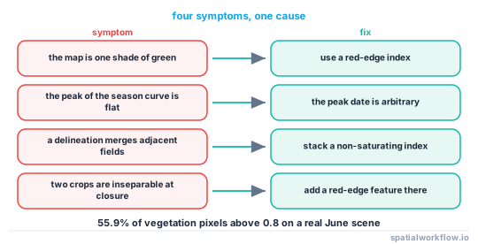
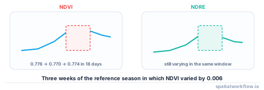
The NDVI map of a field in mid-June is one shade of green. Fields that differ visibly in biomass have the same value, the within-field variation has vanished, and a time series through the peak is a flat line for three weeks.
This is saturation, and it is not a data problem. Chlorophyll absorbs essentially all incident red light once the leaf area index passes about three, so additional leaves change red reflectance almost not at all while near-infrared keeps rising slowly. The normalised difference asymptotes; the canopy does not.
Measured on a cloud-free Sentinel-2 scene over Dutch arable land on 12 June: 64,302 of 114,973 vegetation pixels — 55.9% — were above NDVI 0.8, and across those pixels NDVI varied over a range of 0.128 with a coefficient of variation of 0.032.
Quick answer
Use a red-edge index over the saturated period:
import numpy as np

ndvi = (nir - red) / (nir + red)
ndre = (nir - rededge1) / (nir + rededge1)          # Sentinel-2 B8 and B5

dense = vegetation & (ndvi > 0.8)
for name, arr in (("NDVI", ndvi), ("NDRE", ndre), ("EVI", evi)):
    v = arr[dense]
    print(f"{name:5} range {v.max()-v.min():.3f}  sd {v.std():.4f}  "
          f"CV {v.std()/abs(v.mean()):.3f}")
NDVI range 0.128 sd 0.0278 CV 0.032
NDRE range 0.572 sd 0.0644 CV 0.098
EVI range 0.684 sd 0.0807 CV 0.106
Three times the relative variation from NDRE on identical ground. Across 101 fields whose median NDVI exceeded 0.8, NDVI spanned 0.102 between fields and NDRE spanned 0.264.
Step-by-step solution
1. Confirm it is saturation and not a masking problem
Saturation shows as a high, narrow distribution: most vegetation pixels above 0.8 with a small spread. A masking problem shows as a bimodal distribution with a cloud or shadow population.
2. Measure how much of the season is affected
The field-median NDVI on the reference series sat at 0.776, 0.770 and 0.774 on 12, 18 and 30 June — three observations spanning eighteen days with a total range of 0.006. That whole period contributes nothing to any analysis based on NDVI.
3. Switch to a red-edge index for the saturated window
Sentinel-2 band 5 at 705 nm sits on the steep part of the vegetation reflectance curve, where absorption is partial and further chlorophyll still changes reflectance.
4. Use the right red-edge band
Band 7 at 783 nm is already on the NIR plateau, so the normalised difference against NIR collapses towards zero. On the same scene, the median NDRE was +0.587 with band 5 and +0.018 with band 7.
5. Consider EVI if you have a reliable blue band
EVI performed comparably to NDRE on the dense pixels — a range of 0.684 and a CV of 0.106 — and it is available on sensors with no red edge. Its weakness is that it depends on the blue band, whose atmospheric correction is the least reliable.
6. Fix the downstream consequences
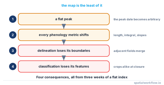
Saturation does not only flatten the map. It flattens the peak of a phenology curve, so the peak date becomes arbitrary; it removes the boundaries a field delineation depends on; and it removes the feature that separates two crops at full canopy.
7. Keep NDVI for the parts of the season where it works
Emergence, early growth and senescence are all well below saturation, and NDVI's cross-sensor consistency there is worth keeping. The fix is to use both, not to abandon one.
Code examples
Example 1 — quantify the saturation on your own scene
import numpy as np

def saturation_report(ndvi, ndre, evi, vegetation_mask, threshold=0.8):
    veg = vegetation_mask & np.isfinite(ndvi) & np.isfinite(ndre)
    dense = veg & (ndvi > threshold)
    out = {"vegetation_pixels": int(veg.sum()),
           "dense_pixels": int(dense.sum()),
           "dense_share": round(float(dense.sum() / veg.sum()), 3)}
    for name, arr in (("ndvi", ndvi), ("ndre", ndre), ("evi", evi)):
        v = arr[dense]
        v = v[np.isfinite(v)]
        out[f"{name}_range"] = round(float(v.max() - v.min()), 3)
        out[f"{name}_sd"] = round(float(v.std()), 4)
        out[f"{name}_cv"] = round(float(v.std() / abs(v.mean())), 3)
    out["ndre_advantage"] = round(out["ndre_cv"] / out["ndvi_cv"], 2)
    return out

print(saturation_report(ndvi, ndre, evi, scl == 4))
{'vegetation_pixels': 114973, 'dense_pixels': 64302, 'dense_share': 0.559,
'ndvi_range': 0.128, 'ndvi_sd': 0.0278, 'ndvi_cv': 0.032,
'ndre_range': 0.572, 'ndre_sd': 0.0644, 'ndre_cv': 0.098,
'evi_range': 0.684, 'evi_sd': 0.0807, 'evi_cv': 0.106, 'ndre_advantage': 3.06}
Example 2 — separation between fields, which is what usually matters
import numpy as np, pandas as pd

def field_separation(field_table, threshold=0.8):
    hi = field_table[field_table["ndvi"] > threshold]
    print(f"{len(hi)} of {len(field_table)} fields above NDVI {threshold}")
    for col in ("ndvi", "ndre"):
        print(f"  {col.upper():5} spread between fields "
              f"{hi[col].max() - hi[col].min():.3f}, sd {hi[col].std():.4f}")
    print(f"  within-field CV: NDVI median {hi['ndvi_cv'].median():.3f}, "
          f"NDRE median {hi['ndre_cv'].median():.3f}")
    return hi
101 of 161 fields above NDVI 0.8
NDVI spread between fields 0.102, sd 0.0246
NDRE spread between fields 0.264, sd 0.0549
within-field CV: NDVI median 0.128, NDRE median 0.138
Between fields, NDRE separates 2.6 times better. Within fields the two are similar, which is worth knowing: saturation costs most when comparing fields, and less when mapping variation inside one.
Example 3 — a season stack that switches index by growth stage
import numpy as np, pandas as pd

def blended_index(dates, ndvi, ndre, saturate_at=0.75):
    """Use NDVI while it is informative and NDRE once it saturates."""
    out, source = [], []
    for d, a, b in zip(dates, ndvi, ndre):
        if np.nanmedian(a) > saturate_at:
            out.append(b)
            source.append("ndre")
        else:
            out.append(a)
            source.append("ndvi")
    return np.array(out), pd.Series(source, index=pd.DatetimeIndex(dates))

blend, src = blended_index(season.date, season.ndvi_med, season.ndre_med)
print(src.value_counts().to_string())
Blending is a pragmatic choice rather than a principled one — the two indices are on different scales — so it suits a segmentation or a classifier feature far better than it suits a published time series. For a published series, report both.
Explanation
Why absorption is the limit
Red light is absorbed by chlorophyll. A canopy with a leaf area index of one already absorbs most of the red incident on it; by three, essentially all of it. Further leaves therefore cannot lower red reflectance any further, so the numerator nir − red grows only as fast as NIR, and the denominator grows at the same rate. The ratio flattens.
Why the red edge keeps responding
Between roughly 700 and 730 nm, chlorophyll absorption is falling steeply and is only partial even in a dense canopy. Additional chlorophyll still reduces reflectance measurably there, so a normalised difference against NIR keeps varying. That is also why red-edge indices track leaf nitrogen: the relationship is with chlorophyll concentration rather than merely with cover.
Why band 7 does not work
By 783 nm the leaf's absorption has essentially stopped and reflectance is on the NIR plateau, close to band 8's value. The normalised difference between two similar values is near zero and carries little information — hence the +0.018 median against +0.587 for band 5.
Why the downstream effects are larger than the map
A flat peak makes the peak date arbitrary, which propagates into every phenology metric. It removes the between-field contrast that a delineation needs, causing adjacent fields to merge. And it removes the biomass differences that separate two cereals at full canopy, which is where a crop classifier makes most of its errors. The flat map is the least of it.
Edge cases or notes
- The threshold is not universal. 0.8 suits temperate arable; check your own distribution.
- Shadow looks like dense canopy to every index. Mask it.
- Band resolutions differ. Red and NIR are 10 m; the red edges are 20 m.
- Not every sensor has a red edge. Landsat does not; use EVI there.
- EVI depends on the blue band, whose atmospheric correction is least reliable.
- Saturation is worse at nadir and varies with sun angle.
- NDVI is still right for emergence and senescence. Use both.
- State which index each figure used. They are not on the same scale.
Internal links
- Vegetation indices explained: NDVI, EVI, NDRE and when each fails — the whole family
- Crop phenology and growing seasons explained — the flat peak
- How to extract phenology metrics from an NDVI time series — the arbitrary peak date
- Delineated field boundaries merge fields or swallow roads — the missing boundaries
- A crop classifier confuses two crops every year — the missing separation
- Spectral indices explained — the wider context
- How to calculate NDVI in Python — the basic computation
- NDVI values are out of range — a different NDVI problem
FAQ
Why is my NDVI map all one colour in summer?
Saturation. On a real June scene, 55.9% of vegetation pixels were above 0.8 and varied over a range of only 0.128.
What should I use instead?
A red-edge index — NDRE from Sentinel-2 bands 8 and 5 — or EVI. On the same pixels NDRE varied over 0.572 and EVI over 0.684.
Which red-edge band?
Band 5 at 705 nm. Band 7 at 783 nm is already on the NIR plateau and gave a median NDRE of +0.018 against +0.587 for band 5.
Does saturation matter within a field or between fields?
Mostly between. Across 101 dense fields, NDRE separated them 2.6 times better than NDVI; within fields the two were similar.
What if my sensor has no red-edge band?
Use EVI, which was comparable to NDRE on the dense pixels — at the cost of depending on the blue band's atmospheric correction.
Should I stop using NDVI?
No. It works well at emergence and senescence and has unmatched cross-sensor consistency. Use it where it responds and something else where it does not.