
How to clean yield monitor data in Python
Problem statement
Raw yield monitor data is a track log with a yield column, and the artefacts in it are structural rather than random: start and stop transients at the end of every pass, inflated or deflated values wherever the header was not full, a ten-to-twenty-second sensor lag that smears every boundary, and a scattering of physically impossible values.
Cleaning is therefore not outlier removal. It is a sequence of rules, each targeting a known mechanism, applied in an order that matters — and the count removed by each rule is part of the result, because a pipeline that silently discards a quarter of the points has made a decision nobody reviewed.
Quick answer
import numpy as np, pandas as pd

def clean_yield(y, lag_s=12, min_speed=1.5, max_speed=12, trim_points=8,
                full_swath=None, yield_range=(0.5, 25)):
    n0 = len(y)
    log = {}

    y = y.sort_values("timestamp").copy()
    y = add_pass_id(y)
    y = correct_lag(y, lag_s)

    keep = y["from_end"].ge(trim_points) & y["point_in_pass"].ge(trim_points)
    log["start_stop"] = int((~keep).sum()); y = y[keep]

    keep = y["speed_kmh"].between(min_speed, max_speed)
    log["speed"] = int((~keep).sum()); y = y[keep]

    if full_swath is not None:
        keep = y["swath_m"] >= 0.95 * full_swath
        log["partial_width"] = int((~keep).sum()); y = y[keep]

    keep = y["yield_lag_corrected"].between(*yield_range)
    log["impossible"] = int((~keep).sum()); y = y[keep]

    print(f"{n0:,} → {len(y):,} points ({len(y)/n0:.1%} kept)")
    print(pd.Series(log).to_string())
    return y, log
Every rule reports. If partial_width removes 30% of the points, that is a fact about the field's shape, not a bug — but it is a fact that belongs in the output.
Step-by-step solution
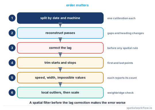
1. Split by harvest date and by machine first
A file can contain two harvests or two combines. Each has its own calibration, its own lag and its own swath, and mixing them makes every later rule wrong.
2. Reconstruct the passes
A pass ends where there is a time gap or a large heading change. Everything afterwards — trimming, headland detection, lag correction — operates within a pass.
3. Correct the lag before any spatial rule
The lag displaces values along the track by tens of metres. Applying a spatial filter first smooths the displaced values and then displaces them again, which makes the error worse rather than better.
4. Trim the start and stop of every pass
Flow builds and decays over several seconds. Dropping the first and last six to ten points of each pass removes the transients; the exact number depends on the logging interval and the machine.
5. Filter speed
Very low speeds give division by a small number; very high speeds are transport between fields. Both produce spikes.
6. Handle partial width
Where the logged swath is below the full header width, the area is wrong and so is the yield. If the true swath is logged, correct it; if it is not, remove the points.
7. Remove physically impossible values, then statistical outliers
A negative yield or 60 t/ha of wheat is impossible. After the impossible values are gone, a local outlier rule — a median absolute deviation within a moving neighbourhood — catches the rest without being dominated by them.
8. Scale to the weighbridge
The sum of the cleaned map should match the delivered tonnage. Applying a single scale factor to match it is standard practice and is the only external check available.
Code examples
Example 1 — passes, lag and trimming
import numpy as np, pandas as pd

def add_pass_id(y, gap_s=10, turn_deg=60):
    y = y.sort_values("timestamp").copy()
    dt = y["timestamp"].diff().dt.total_seconds()
    turn = y["heading_deg"].diff().abs().mod(360)
    turn = np.minimum(turn, 360 - turn)
    y["pass_id"] = ((dt > gap_s) | (turn > turn_deg)).cumsum()
    y["point_in_pass"] = y.groupby("pass_id").cumcount()
    y["from_end"] = (y.groupby("pass_id")["point_in_pass"].transform("max")
                     - y["point_in_pass"])
    return y

def correct_lag(y, lag_s=12.0, col="yield_t_ha"):
    out = []
    for _, g in y.groupby("pass_id", sort=False):
        g = g.sort_values("timestamp").copy()
        t = (g["timestamp"] - g["timestamp"].iloc[0]).dt.total_seconds().values
        g["yield_lag_corrected"] = np.interp(t, t - lag_s, g[col].values,
                                             left=np.nan, right=np.nan)
        out.append(g)
    return pd.concat(out)
Example 2 — estimate the lag rather than assuming it
import numpy as np

def estimate_lag(y, boundary_geom, candidates=np.arange(0, 25, 1.0)):
    """Choose the lag that makes the yield step align with a known boundary."""
    best, best_score = None, -np.inf
    inside = y.geometry.within(boundary_geom)
    for lag in candidates:
        shifted = correct_lag(y, lag)["yield_lag_corrected"]
        a, b = shifted[inside.values], shifted[~inside.values]
        a, b = a[np.isfinite(a)], b[np.isfinite(b)]
        if len(a) < 50 or len(b) < 50:
            continue
        # t-like separation: a sharp boundary maximises it
        score = abs(a.mean() - b.mean()) / np.sqrt(a.var() / len(a) + b.var() / len(b))
        if score > best_score:
            best, best_score = lag, score
    print(f"best lag {best:.1f} s (separation {best_score:.1f})")
    return best
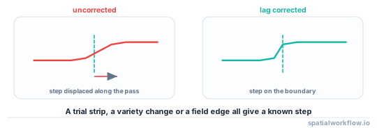
A trial strip, a variety change or a field boundary all give a known step. Estimating the lag once per combine is worth far more than using a default, because the default is wrong by enough to matter.
Example 3 — local outliers and the weighbridge scale
import numpy as np, geopandas as gpd
from scipy.spatial import cKDTree

def local_outliers(y, col="yield_lag_corrected", k=20, mad_threshold=3.5):
    xy = np.c_[y.geometry.x, y.geometry.y]
    tree = cKDTree(xy)
    _, idx = tree.query(xy, k=k + 1, workers=-1)
    v = y[col].values
    neigh = v[idx[:, 1:]]
    med = np.nanmedian(neigh, axis=1)
    mad = np.nanmedian(np.abs(neigh - med[:, None]), axis=1)
    score = 0.6745 * (v - med) / np.where(mad == 0, np.nan, mad)
    flag = np.abs(score) > mad_threshold
    print(f"local outliers: {np.nansum(flag):,} of {len(y):,} "
          f"({np.nansum(flag)/len(y):.1%})")
    return y[~np.nan_to_num(flag, nan=False)]

def scale_to_weighbridge(y, delivered_t, area_ha, col="yield_lag_corrected"):
    mapped = y[col].mean() * area_ha
    factor = delivered_t / mapped
    print(f"map total {mapped:.1f} t, delivered {delivered_t:.1f} t, "
          f"scale factor {factor:.3f}")
    y = y.copy()
    y["yield_scaled"] = y[col] * factor
    return y, factor
A scale factor far from 1 — outside roughly 0.9 to 1.1 — means the calibration or the swath assumption is wrong, and scaling it away hides a problem that will recur next year.
Explanation
Why the order of the rules matters
The lag correction moves values along the track, so it must come before anything that depends on position — local outlier detection, headland masking, rasterising. Pass reconstruction must come before trimming, because "the first eight points" is meaningless without a pass. Removing impossible values before the statistical rule stops a handful of 400 t/ha points from setting the threshold for everything else.
Why partial-width points are removed rather than corrected
The monitor divides measured mass by assumed area. If the true swath was logged, the correction is arithmetic. If it was not — which is common on older monitors — there is no information from which to recover the area, and the value is simply wrong by an unknown factor. Removing them loses coverage along one edge of the field and keeps the rest honest.
Why a local rule beats a global one
Yield varies across a field by a factor of two or more, so a global threshold either keeps outliers in the low-yielding part or removes real data from the high-yielding part. Comparing each point with its twenty nearest neighbours adapts to the local level, and the median absolute deviation makes it robust to the outliers it is looking for.
Why the weighbridge is the only external check
Everything else in a yield map is internally consistent by construction: the monitor's calibration, the swath assumption and the moisture correction all affect the whole map together, so no internal statistic reveals them. The delivered tonnage is measured independently, and the ratio between it and the map total is the one number that tests the whole chain.
Edge cases or notes
- Split by date and machine first. Everything downstream assumes one of each.
- The lag is a machine property. Estimate it once, reuse it.
- Headlands may deserve their own treatment rather than deletion.
- Overlap between passes double-counts. Detect it geometrically if the swath is logged.
- Moisture basis must be consistent before any comparison between passes.
- Keep the removed points. They are the evidence for the cleaning report.
- A scale factor outside 0.9–1.1 is a warning, not a correction.
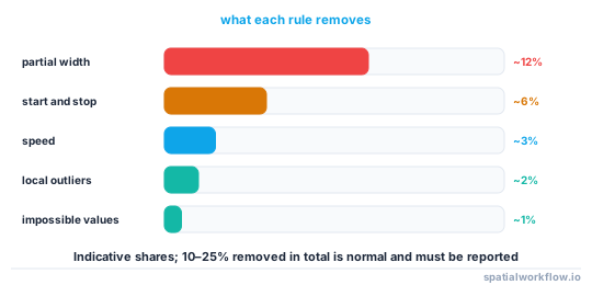
- Report the kept fraction. Twenty per cent removed is normal and should be visible.
Internal links
- Yield monitor data explained: what the numbers really are — where each artefact comes from
- A yield map has impossible values and stripes — diagnosing before cleaning
- How to remove spatial outliers in Python — the local rule in general
- Management zones explained — what the cleaned map feeds
- How to clean a GPS track in Python — pass reconstruction
- How to calculate speed, distance and direction along a track — the speed filter
- How to analyse an on-farm strip trial in Python — where the lag limits resolution
- Repair, reject or flag — deciding what to do with bad rows
FAQ
How much yield data should I expect to remove?
Ten to twenty-five per cent for a defensible pass. Report the count removed by each rule.
What order should the cleaning rules go in?
Split by date and machine, reconstruct passes, correct the lag, trim starts and stops, filter speed, handle partial width, remove impossible values, then local outliers.
How do I find the sensor lag?
Sweep candidate lags and pick the one that maximises the separation across a known boundary — a trial strip, a variety change or a field edge.
Should I correct or remove partial-width points?
Correct them if the true swath was logged. If it was not, the area is unrecoverable and the points have to go.
Why use a local outlier rule?
Because yield varies across a field by a factor of two, so a global threshold removes real data in the good areas and keeps outliers in the poor ones.
What does the weighbridge check tell me?
Whether the whole chain — calibration, swath, moisture — is right. A scale factor outside about 0.9 to 1.1 is a problem to fix, not to scale away.