
Management zones explained
Problem statement
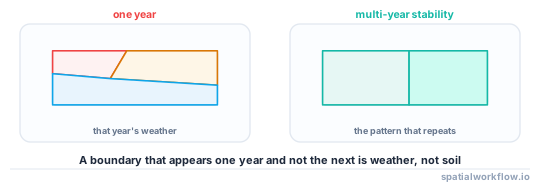
A management zone is a part of a field that is treated differently — a different seed rate, a different nitrogen rate, a different sampling density. The idea is old and the failure is consistent: zones drawn from one year's yield map, or from one satellite image, describe that year's weather rather than the field's persistent character.
The test that matters is stability. A zone boundary that appears in 2022, disappears in 2023 and reappears in 2024 is noise; one that appears every year is a soil boundary, a drainage line or a compaction pattern, and is worth acting on.
This guide covers what to build zones from, how many to make, and how to decide whether they mean anything.
Quick answer
Build zones from several years of a stable layer, then test the separation:
import numpy as np
from sklearn.cluster import KMeans
from sklearn.preprocessing import StandardScaler

X = StandardScaler().fit_transform(np.c_[ndvi_2023, ndvi_2024, ndvi_2025, elevation, ec_shallow])
labels = KMeans(n_clusters=3, n_init=20, random_state=0).fit_predict(X)

# does the zoning explain anything?
ss_total = ((yield_ - yield_.mean()) ** 2).sum()
ss_within = sum(((yield_[labels == k] - yield_[labels == k].mean()) ** 2).sum()
                for k in np.unique(labels))
print(f"variance explained by the zoning: {1 - ss_within / ss_total:.1%}")
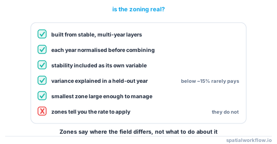
If the zoning explains a few percent of the yield variance, it is not a zoning. The threshold is a judgement — in practice, below about 15% the zones rarely pay for the complexity they add.
Step-by-step solution
1. Prefer layers that do not change between years
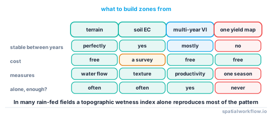
- Elevation and terrain derivatives — slope, curvature, topographic wetness. Free, perfectly stable, and often the strongest single predictor.
- Apparent soil electrical conductivity — a proxy for texture and depth. Stable, and needs a survey.
- Multi-year vegetation index composites — the mean and, more usefully, the stability of an index over several seasons.
- Soil survey polygons — stable and usually too coarse.
- A single yield map — the least stable thing on the list.
2. Normalise each year before combining
Yield and vegetation indices differ between years in absolute level. Converting each year to a within-field z-score or a percentile removes the season and leaves the pattern, which is the thing zones are supposed to capture.
3. Use both the mean and the variability
The mean tells you where the field is good; the temporal standard deviation tells you where it is reliable. A part of the field that is consistently mediocre and one that alternates between excellent and terrible need different management, and a mean-only zoning puts them together.
4. Choose the number of zones from the data and the machinery
Two or three is usual. More zones need more evidence to justify and more work to manage, and most spreaders and drills have a limited number of rates they can hold anyway.
5. Smooth and simplify the result
Raw cluster output is speckled and no machine can follow it. A modal filter, a minimum zone area and a simplification tolerance appropriate to the boom width turn it into something a controller can drive.
6. Validate against an independent year
Fit the zones on some years, test whether they separate yield in a year that was not used. That is the only check that distinguishes a real pattern from an elaborate description of noise.
7. Expect zones to fail on the things that matter most
A zoning built from productivity does not know about a nitrogen response. A part of the field that yields poorly because it is thin soil needs less nitrogen; one that yields poorly because it is waterlogged may need drainage rather than any rate at all. Zones tell you where the field differs, not what to do about it.
Code examples
Example 1 — normalise, stack and cluster
import numpy as np, pandas as pd
from sklearn.cluster import KMeans
from sklearn.preprocessing import StandardScaler

def build_layers(years: dict, extra: dict = None):
    """years: {label: array}. Each year is converted to a within-field z-score."""
    stack = {}
    for label, arr in years.items():
        a = np.asarray(arr, dtype="float32")
        stack[f"z_{label}"] = (a - np.nanmean(a)) / np.nanstd(a)
    z = np.stack(list(stack.values()))
    stack["mean_z"] = np.nanmean(z, axis=0)
    stack["stability"] = -np.nanstd(z, axis=0)        # high = consistent
    for k, v in (extra or {}).items():
        a = np.asarray(v, dtype="float32")
        stack[k] = (a - np.nanmean(a)) / np.nanstd(a)
    return stack

def zones(stack, k=3, use=("mean_z", "stability", "elevation")):
    cols = [stack[c].ravel() for c in use if c in stack]
    X = np.column_stack(cols)
    ok = np.isfinite(X).all(axis=1)
    labels = np.full(X.shape[0], -1, dtype="int16")
    km = KMeans(n_clusters=k, n_init=20, random_state=0).fit(X[ok])
    labels[ok] = km.labels_
    # order the zones by mean productivity so zone 0 is always the poorest
    order = np.argsort([stack["mean_z"].ravel()[labels == i].mean() for i in range(k)])
    remap = {old: new for new, old in enumerate(order)}
    labels[ok] = np.vectorize(lambda v: remap[v])(labels[ok])
    return labels.reshape(stack["mean_z"].shape)
Ordering the zones by productivity is a small thing that saves a great deal of confusion: without it, zone 1 means something different every time the clustering is re-run.
Example 2 — test whether the zoning explains anything
import numpy as np, pandas as pd

def zone_quality(labels, target, min_cells=30):
    lab, y = labels.ravel(), np.asarray(target).ravel()
    ok = (lab >= 0) & np.isfinite(y)
    lab, y = lab[ok], y[ok]

    ss_total = ((y - y.mean()) ** 2).sum()
    rows, ss_within = [], 0.0
    for k in np.unique(lab):
        v = y[lab == k]
        if len(v) < min_cells:
            continue
        ss_within += ((v - v.mean()) ** 2).sum()
        rows.append({"zone": int(k), "cells": len(v), "share": len(v) / len(y),
                     "mean": float(v.mean()), "sd": float(v.std())})
    df = pd.DataFrame(rows)
    return df, {"variance_explained": float(1 - ss_within / ss_total),
                "separation": float(df["mean"].max() - df["mean"].min()),
                "smallest_zone_share": float(df["share"].min())}
Three numbers decide it: how much variance the zoning explains, how far apart the zone means are, and whether the smallest zone is large enough to manage.
Example 3 — smooth into something a machine can drive
import numpy as np, geopandas as gpd
from scipy import ndimage
from rasterio.features import shapes
from shapely.geometry import shape

def zones_to_polygons(labels, transform, crs, min_area_ha=1.0, modal_size=5,
                      simplify_m=None, boom_width_m=24):
    smooth = ndimage.median_filter(labels.astype("int16"), size=modal_size)
    polys = []
    for geom, val in shapes(smooth, mask=smooth >= 0, transform=transform):
        polys.append({"zone": int(val), "geometry": shape(geom)})
    g = gpd.GeoDataFrame(polys, crs=crs).dissolve("zone", as_index=False).explode(index_parts=False)
    g["area_ha"] = g.area / 1e4
    g = g[g.area_ha >= min_area_ha]
    g["geometry"] = g.geometry.simplify(simplify_m or boom_width_m / 2)
    return g.dissolve("zone", as_index=False)
Simplifying at half the boom width is the right order of magnitude: detail finer than the implement cannot be applied, so keeping it only makes the file larger and the controller's job harder.
Explanation
Why a single year's yield map makes poor zones
Yield in any one year is the product of the field's persistent character and that season's weather, management and pest pressure. In a dry year the light land yields poorly; in a wet year it yields best. A zoning fitted to one year therefore encodes a weather interaction, and applying it in a year with different weather can be worse than a uniform rate.
Why stability deserves its own layer
Two parts of a field can have the same multi-year mean and completely different behaviour: one steady, one alternating. The steady part responds predictably to a rate change; the variable part is being limited by something that varies — water, usually — and a fixed rate for it is a guess. Including the temporal standard deviation as a clustering input separates them.
Why terrain is so often the strongest input
Elevation, slope and curvature drive water movement, and water is the dominant limitation in most rain-fed systems. Terrain is also free, perfectly stable and available at high resolution. In many fields a topographic wetness index alone reproduces most of a multi-year yield pattern.
Why zones are a description and not a prescription
Clustering tells you where the field differs. It does not tell you whether a poor area is poor because of nitrogen, water, compaction, pH or pests, and the correct rate response differs — sometimes in opposite directions — between those causes. Turning zones into rates needs an agronomic model or an on-farm trial, which is why How to analyse an on-farm strip trial in Python exists.
Edge cases or notes
- Normalise per year, always. Absolute levels differ between seasons.
- Order the zones by productivity so the labels mean the same thing each run.
- Two zones are often enough. More needs more evidence.
- Headlands behave differently from the field centre and are often their own zone.
- Very small zones cannot be managed. Set a minimum area.
- Machinery has a rate resolution. Zones finer than it are wasted.
- Test on a held-out year. Fitting and testing on the same years proves nothing.
- Record the input layers and years with the zone map.
Internal links
- How to build management zones with clustering in Python — the implementation
- Yield monitor data explained: what the numbers really are — why one year's map is unstable
- How to write a variable-rate prescription map — turning zones into rates
- How to analyse an on-farm strip trial in Python — finding the response the zones cannot
- Spatial clustering explained — the clustering underneath
- How to calculate slope and aspect in Python — the terrain inputs
- How to lay out a soil sampling grid in Python — sampling by zone
- Field boundary data explained: where it comes from — the field the zones subdivide
FAQ
What is a management zone?
A part of a field that is managed differently — a different seed, nutrient or irrigation rate — because it behaves differently from the rest.
What should I build zones from?
Stable layers: terrain, soil electrical conductivity and a multi-year vegetation index composite. A single year's yield map is the least stable option.
How many zones should I make?
Two or three in most cases. More zones need more evidence to justify and more rates than most machinery can hold.
How do I know the zones are real?
Fit them on some years and test whether they separate yield in a year you held out. Also report the variance explained; below about 15% they rarely earn their complexity.
Why include a stability layer?
Because a consistently mediocre area and an alternately excellent and terrible one need different management, and a mean-only zoning merges them.
Do zones tell me what rate to apply?
No. They tell you where the field differs. The rate response needs an agronomic model or an on-farm trial.