
How to analyse an on-farm strip trial in Python
Problem statement
A strip trial is the only way to measure how a field responds to a rate change, and the statistics are harder than they look. Yield varies across a field by more than most treatment effects, so a treated strip that happens to lie on the better land shows a response that is the land, not the treatment.
Two things fix it. Pairing each treated strip with its immediate neighbours removes most of the spatial trend, because adjacent strips share their soil. And a test that accounts for spatial autocorrelation gives an honest standard error, because yield points a few metres apart are not independent observations — treating 20,000 of them as independent makes almost any difference significant.
Quick answer
Compare each treated strip with its neighbours, then test on strip means:
import numpy as np, pandas as pd
from scipy import stats

paired = []
for s in treated_strips:
    t = yields[yields.strip_id == s]["yield_t_ha"].mean()
    c = yields[yields.strip_id.isin(neighbours[s])]["yield_t_ha"].mean()
    paired.append({"strip": s, "treated": t, "control": c, "diff": t - c})

p = pd.DataFrame(paired)
res = stats.ttest_rel(p["treated"], p["control"])
print(f"{len(p)} pairs; mean difference {p['diff'].mean():+.3f} t/ha "
      f"(sd {p['diff'].std():.3f}), p = {res.pvalue:.3f}")
The degrees of freedom are the number of strip pairs, not the number of yield points. Eight pairs is eight observations however many million data points the combine recorded.
Step-by-step solution
1. Lay the trial out so it can be analysed
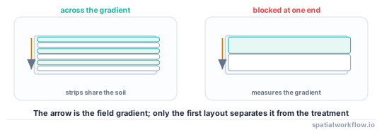
Strips the width of the harvester (or a multiple), running across the dominant gradient, alternating or replicated, with at least six to eight replicates. A design with two strips cannot be analysed however good the statistics.
2. Clean the yield data first
Lag correction, start and stop trimming, partial-width removal. The sensor lag alone smears the boundary between strips by tens of metres, which is a large fraction of a strip width — see Yield monitor data explained.
3. Trim the strip edges
Overlap between passes, spreader overlap and the lag all contaminate the first and last few metres of each strip. Buffering each strip inwards by a few metres before extracting the yield removes it.
4. Aggregate to strip means before testing
Each strip is one experimental unit. Testing on individual yield points treats 20,000 correlated observations as independent and produces a p-value that is meaningless.
5. Pair with neighbours rather than pooling
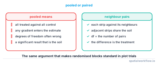
The mean of all treated strips against the mean of all control strips is vulnerable to any gradient across the field. Comparing each treated strip with the mean of its immediate neighbours removes most of it.
6. Check the residual spatial structure
If the differences still show a spatial pattern, the pairing has not removed the trend and a spatial model — a linear mixed model with a spatial correlation structure, or simply including position as a covariate — is needed.
7. Report the effect size and the interval, not just the p-value
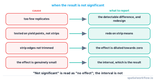
A difference of 0.12 t/ha with a 95% interval from −0.20 to +0.44 is a result: the trial could not detect anything smaller than about half a tonne. That is more useful than "not significant".
Code examples
Example 1 — extract strip yields with the edges trimmed
import numpy as np, geopandas as gpd, pandas as pd

def strip_yields(yields, strips, trim_m=5, min_points=100):
    s = strips.copy()
    s["geometry"] = s.geometry.buffer(-trim_m)
    s = s[~s.geometry.is_empty]

    j = gpd.sjoin(yields, s[["strip_id", "treatment", "geometry"]],
                  predicate="within", how="inner")
    g = j.groupby(["strip_id", "treatment"])["yield_t_ha"].agg(
        ["count", "mean", "std"]).reset_index()
    dropped = g[g["count"] < min_points]
    if len(dropped):
        print(f"dropping {len(dropped)} strips with fewer than {min_points} points")
    g = g[g["count"] >= min_points]
    print(g.groupby("treatment")[["count", "mean"]].agg(
        {"count": "sum", "mean": "mean"}).round(3).to_string())
    return g
Example 2 — neighbour pairing and the paired test
import numpy as np, pandas as pd, geopandas as gpd
from scipy import stats

def neighbour_pairs(strip_stats, strips, treated="high", control="standard"):
    centroids = strips.set_index("strip_id").geometry.centroid
    stats_by_id = strip_stats.set_index("strip_id")

    rows = []
    for sid in strip_stats.query("treatment == @treated")["strip_id"]:
        here = centroids.loc[sid]
        others = strip_stats.query("treatment == @control")["strip_id"]
        d = centroids.loc[others].distance(here).sort_values()
        near = d.index[:2]
        if len(near) < 2:
            continue
        rows.append({"strip_id": sid,
                     "treated": stats_by_id.loc[sid, "mean"],
                     "control": float(stats_by_id.loc[near, "mean"].mean()),
                     "neighbours": list(near)})
    p = pd.DataFrame(rows)
    p["diff"] = p["treated"] - p["control"]
    return p

def paired_result(p, alpha=0.05):
    n = len(p)
    d = p["diff"].values
    t = stats.ttest_rel(p["treated"], p["control"])
    se = d.std(ddof=1) / np.sqrt(n)
    half = stats.t.ppf(1 - alpha / 2, n - 1) * se
    return {"pairs": n, "mean_diff": round(float(d.mean()), 3),
            "sd": round(float(d.std(ddof=1)), 3), "se": round(float(se), 3),
            "ci_low": round(float(d.mean() - half), 3),
            "ci_high": round(float(d.mean() + half), 3),
            "p_value": round(float(t.pvalue), 4),
            "detectable_at_80_power": round(float(2.8 * se), 3)}
detectable_at_80_power is the number worth quoting when the result is not significant: roughly 2.8 standard errors is the difference this trial could have detected, and it tells the farmer whether the trial was worth running.
Example 3 — check the residual spatial structure
import numpy as np, pandas as pd
from scipy.spatial import cKDTree

def residual_autocorrelation(p, strips, k=3):
    """Moran's I on the paired differences: is there structure the pairing missed?"""
    c = strips.set_index("strip_id").geometry.centroid
    xy = np.c_[c.loc[p.strip_id].x, c.loc[p.strip_id].y]
    d = p["diff"].values
    z = d - d.mean()

    tree = cKDTree(xy)
    _, idx = tree.query(xy, k=min(k + 1, len(xy)))
    W = np.zeros((len(xy), len(xy)))
    for i, row in enumerate(idx[:, 1:]):
        W[i, row] = 1
    W = (W + W.T) / 2

    n, s0 = len(z), W.sum()
    I = (n / s0) * (z @ W @ z) / (z @ z)
    expected = -1 / (n - 1)
    print(f"Moran's I on the differences: {I:+.3f} (expected {expected:+.3f})")
    if I > 0.3:
        print("! the pairing has not removed the spatial trend — use a spatial model")
    return float(I)
With eight to twelve pairs the test has little power, so treat it as a warning rather than a decision. A strongly positive value means the differences themselves are spatially clustered, which the pairing was supposed to prevent.
Explanation
Why the pseudo-replication problem is so severe
A combine logs a point every second or so, and a strip 600 m long produces several thousand of them. They are not independent: neighbouring points share soil, weather and the same sensor calibration, and their correlation at short lags is very high. A t-test on the raw points has thousands of degrees of freedom and will report a p-value below 0.001 for a difference of a few kilograms. Aggregating to strip means restores the correct number of experimental units, which is the number of strips.
Why neighbour pairing beats a pooled comparison
Fields have gradients — soil type, drainage, headland effects, previous cropping. If the treated strips are on average slightly further up the gradient, a pooled comparison attributes the gradient to the treatment. Adjacent strips share the local conditions almost exactly, so their difference is close to the treatment effect. This is the same argument that makes randomised block designs standard in plot trials.
Why the edges have to be trimmed
Three effects converge on a strip boundary: the harvester's sensor lag displaces yield by tens of metres along the pass, the spreader or drill has a transition zone of several metres where the rate is changing, and adjacent passes overlap. The first few metres of every strip therefore contain a mixture of both treatments, and including them dilutes the measured effect towards zero.
Why to report the detectable difference
Most on-farm trials cannot detect the effects people hope to find. A trial with eight pairs and a standard error of 0.15 t/ha can detect about 0.42 t/ha at 80% power. If the expected response is 0.2 t/ha, the trial was never going to show it, and saying so is far more useful than reporting a non-significant p-value that gets read as "no effect".
Edge cases or notes
- Six to eight replicates minimum. Fewer cannot support a conclusion.
- Strips must cross the gradient, not run along it.
- Strip width should be a multiple of the harvester width.
- Randomise the assignment, or at least alternate.
- Headlands are their own environment. Exclude or treat separately.
- A single year is a single year. Responses vary with the season.
- Record the as-applied data, not just the prescription.
- Report the detectable difference whenever the result is not significant.
Internal links
- How to clean yield monitor data in Python — the cleaning this depends on
- Yield monitor data explained: what the numbers really are — why the edges are contaminated
- Management zones explained — why zones need a trial to become rates
- How to write a variable-rate prescription map — applying the result
- Spatial autocorrelation explained — why points are not independent
- How to calculate Moran's I in Python — the residual check
- Sample design explained — replication and randomisation
- Spatial leakage explained — the same problem in modelling
FAQ
How do I analyse an on-farm strip trial?
Clean the yield data, trim the strip edges, aggregate to one mean per strip, pair each treated strip with its neighbours, and run a paired test on the strip means.
Why can I not test on the individual yield points?
They are not independent. A strip produces thousands of correlated points, and treating them as independent gives a p-value that is meaningless.
How many strips do I need?
Six to eight replicates of each treatment as a minimum. Fewer cannot support a conclusion whatever the analysis.
Why pair with neighbours instead of pooling?
Because fields have gradients. Adjacent strips share their soil, so their difference is close to the treatment effect; a pooled comparison can attribute the gradient to the treatment.
How much of the strip edge should I trim?
A few metres — enough to clear the application transition, the pass overlap and the harvester's lag smear.
What should I report if the result is not significant?
The effect size, the confidence interval and the difference the trial could have detected at reasonable power. "Not significant" on its own is read as "no effect", which is a different claim.