How to Get ERA5 Reanalysis Data in Python

On this page

Problem statement

ERA5 is the most widely used historical weather dataset in the world: hourly estimates of temperature, wind, rain and dozens of other variables on a 0.25° global grid from 1940 to the present, produced by ECMWF for the Copernicus Climate Change Service. The official route is the Climate Data Store, which needs an account, an API key and a request queue. For many uses there is a faster one. Google publishes the whole archive as a public, analysis-ready Zarr store that xarray opens anonymously and reads lazily, a chunk at a time.

This page opens the ERA5 Zarr store on Google Cloud with xarray, builds a map of one hour over North America, reads a day of values for Washington, D.C., converts the units, checks them against the station at Reagan National Airport, and shows why the store suits maps better than long point series.

Quick answer

Open the store anonymously and select one hour over a region; only the chunks needed are downloaded:

ds = xr.open_zarr(STORE, chunks=None, storage_options={"token": "anon"})
box = ds["2m_temperature"].sel(time="2024-07-15T21:00", latitude=slice(55, 20), longitude=slice(360 - 130, 360 - 60)) - 273.15
print(f"{ds.sizes['time']:,} hourly steps on the time axis; map {box.sizes['latitude']} x {box.sizes['longitude']} cells")
print(f"15 July 2024 21:00 UTC: {float(box.min()):.1f} to {float(box.max()):.1f} °C; Washington cell {float(box.sel(latitude=38.75, longitude=283.0, method='nearest')):.1f} °C")

1,323,648 hourly steps on the time axis; map 141 x 281 cells
15 July 2024 21:00 UTC: 7.1 to 42.5 °C; Washington cell 35.0 °C

The time axis has 1,323,648 hourly steps. The map is 141 by 281 cells, and at 21:00 UTC on 15 July 2024 it ranges from 7.1 to 42.5 °C, with 35.0 °C over Washington.

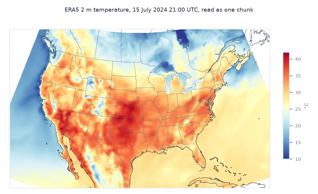
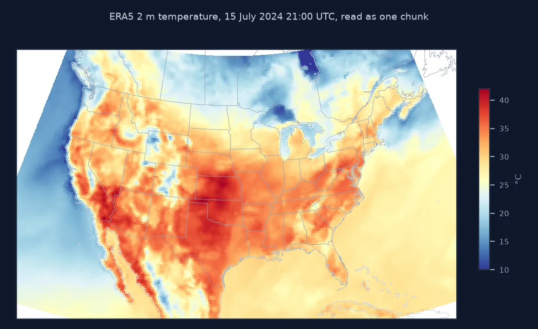
Map of ERA5 2 m temperature over the United States at 21:00 UTC on 15 July 2024, hottest in the southern Plains and the Southwest above 40 °C and cool along the Pacific coast. — One hour, one chunk.

What the store holds, a day at one point, a station check

1. What is in the store

The store holds hundreds of variables, surface and on 37 pressure levels. List the surface ones you are likely to need:

wanted = ["2m_temperature", "2m_dewpoint_temperature", "total_precipitation", "10m_u_component_of_wind", "10m_v_component_of_wind", "surface_pressure"]
for v in wanted:
    print(f"{v:>26}: {ds[v].attrs.get('units', '?'):>4}; dims {ds[v].dims}; chunks {ds[v].encoding.get('chunks')}")
print(f"variables in the store: {len(ds.data_vars)}; the time axis runs to {str(ds.time.values[-1])[:10]}, beyond the data actually filled in")

            2m_temperature:    K; dims ('time', 'latitude', 'longitude'); chunks (1, 721, 1440)
   2m_dewpoint_temperature:    K; dims ('time', 'latitude', 'longitude'); chunks (1, 721, 1440)
       total_precipitation:    m; dims ('time', 'latitude', 'longitude'); chunks (1, 721, 1440)
   10m_u_component_of_wind: m s**-1; dims ('time', 'latitude', 'longitude'); chunks (1, 721, 1440)
   10m_v_component_of_wind: m s**-1; dims ('time', 'latitude', 'longitude'); chunks (1, 721, 1440)
          surface_pressure:   Pa; dims ('time', 'latitude', 'longitude'); chunks (1, 721, 1440)
variables in the store: 273; the time axis runs to 2050-12-31, beyond the data actually filled in

Temperatures are in kelvin, precipitation in metres, wind in m/s and pressure in Pa. Every variable is chunked as one hour of the whole globe, 721 by 1,440 cells. The store has 273 variables, and its time axis runs to 2050, so the last date with data has to be found, not assumed.

2. A day at one point

Each chunk is one hour of the whole globe, so a point series costs one chunk per time step. Read every third hour of 15 July 2024:

pt = ds["2m_temperature"].sel(latitude=38.75, longitude=283.0, method="nearest").sel(time=slice("2024-07-15T00:00", "2024-07-15T21:00", 3))
day = (pt.to_series().astype(float) - 273.15).round(1)
print(day.to_string())
print(f"{len(day)} chunks read for {len(day)} values")

time
2024-07-15 00:00:00    31.8
2024-07-15 03:00:00    28.5
2024-07-15 06:00:00    26.7
2024-07-15 09:00:00    25.0
2024-07-15 12:00:00    28.1
2024-07-15 15:00:00    33.2
2024-07-15 18:00:00    35.7
2024-07-15 21:00:00    35.0
8 chunks read for 8 values

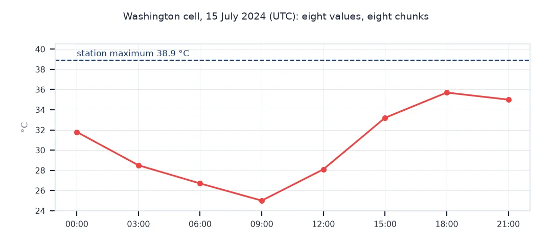
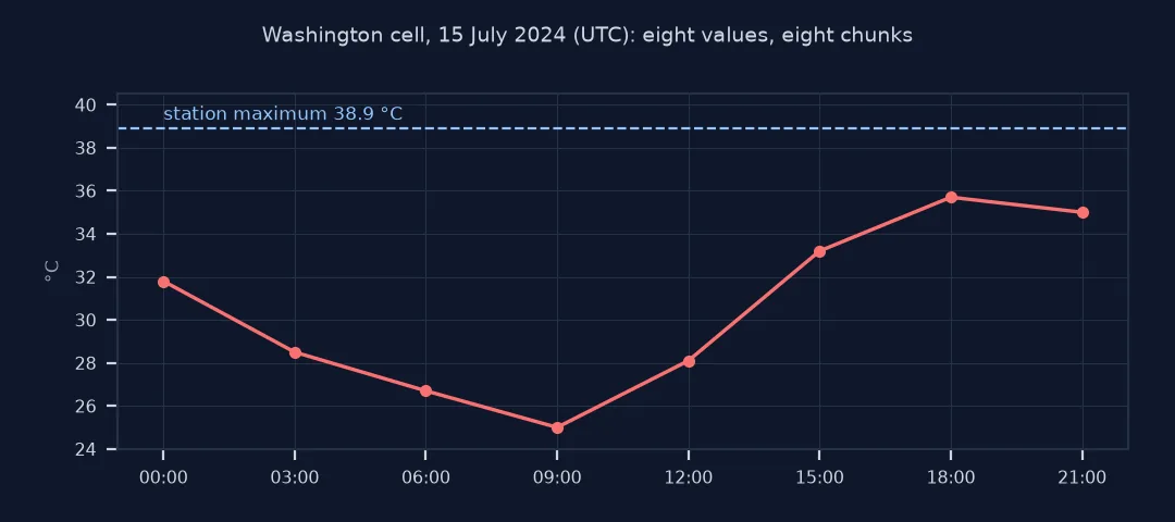
The day's cycle is clear: 25.0 °C at 09:00 UTC, before dawn locally, and 35.7 °C at 18:00 UTC. Each of the 8 values cost one global chunk.

Line chart of ERA5 temperature in the Washington cell every three hours on 15 July 2024, from 25.0 °C at 09:00 UTC to 35.7 °C at 18:00 UTC, below the station maximum of 38.9 °C. — A day at one point.

3. Compare with the station

ERA5 is a grid-cell average. Compare the warmest of those hours with the day's maximum at Reagan National, and the cells around it:

sta = pd.read_csv(GHCN, usecols=["DATE", "TMAX"], parse_dates=["DATE"]).set_index("DATE").TMAX.loc["2024-07-15"] / 10
near = box.sel(latitude=slice(39.5, 38.0), longitude=slice(282.25, 283.75))
print(f"station TMAX 15 July 2024: {sta:.1f} °C; ERA5 cell, warmest 3-hourly value: {day.max():.1f} °C")
print(f"the 7 x 7 cells around Washington at 21:00 UTC: {float(near.min()):.1f} to {float(near.max()):.1f} °C")

station TMAX 15 July 2024: 38.9 °C; ERA5 cell, warmest 3-hourly value: 35.7 °C
the 7 x 7 cells around Washington at 21:00 UTC: 30.7 to 36.3 °C

The station's maximum was 38.9 °C, against 35.7 °C for the warmest 3-hourly value of the cell. Part of the gap is the coarse time sampling, and part is the cell average: the 49 cells around Washington range from 30.7 to 36.3 °C, and none reaches the station value.

Where the store is fast and where it is slow

The data used on this page

ERA5 hourly data on single and pressure levels (Copernicus Climate Change Service), in Google's ARCO-ERA5 analysis-ready Zarr store, public on Google Cloud Storage, opened with xarray and gcsfs; and the GHCN-Daily record for Reagan National Airport (USW00013743) for the comparison.

from pathlib import Path

import pandas as pd
import requests
import xarray as xr

Path("data").mkdir(exist_ok=True)
STORE = "gs://gcp-public-data-arco-era5/ar/full_37-1h-0p25deg-chunk-1.zarr-v3"
GHCN = Path("data/USW00013743.csv")
if not GHCN.exists():
    r = requests.get("https://www.ncei.noaa.gov/data/global-historical-climatology-network-daily/access/USW00013743.csv", timeout=600)
    r.raise_for_status()
    GHCN.write_bytes(r.content)
print(f"xarray {xr.__version__}")

xarray 2026.7.0

The code below uses xarray 2026.7.0.

Example 1: where the store is fast and where it is slow

Time one map and one short point series, and convert to a cost per value:

import time
t0 = time.perf_counter(); _ = float(ds["2m_temperature"].sel(time="2024-07-16T21:00").mean()); t_map = time.perf_counter() - t0
t0 = time.perf_counter(); _ = ds["2m_temperature"].sel(latitude=38.75, longitude=283.0, method="nearest").sel(time=slice("2024-07-16T00:00", "2024-07-16T03:00")).values; t_pt = time.perf_counter() - t0
print(f"one global map: {ds.sizes['latitude'] * ds.sizes['longitude']:,} values from one chunk")
print(f"four hours at one point: 4 values from four chunks; the map costs less than five times the point series: {t_map < 5 * t_pt}")

one global map: 1,038,240 values from one chunk
four hours at one point: 4 values from four chunks; the map costs less than five times the point series: True

A global map is 1,038,240 values from a single chunk, while four hours at one point need four chunks, and the map is cheaper than five times the point series. The store is built for maps. For long point series, use the Open-Meteo archive or a time-chunked copy.

One chunk is one global hour.

What a reanalysis is

Maps fast, point series slow.

ERA5 is a reanalysis. ECMWF runs a modern weather model over the past, assimilating every available observation, from surface stations, radiosondes and aircraft to satellites, to produce the best estimate of the atmosphere's state for every hour since 1940. The result is consistent in space and time and has no gaps, which is why it underlies so much climate and energy research. Its values are averages over 0.25° cells, about 28 by 22 km at Washington. They follow stations closely for temperature on average but smooth out local extremes, and they are weakest for precipitation, which the model produces rather than observes.

The ARCO-ERA5 store reorganises ERA5 as Zarr: compressed chunks of a known shape in cloud storage, read over HTTP on demand. In this version each chunk is one hour of the full global grid, so a map of one hour is a single read, while a long series for one point touches one chunk per hour. That is fine for weeks, slow for decades. For long point series, the Open-Meteo archive or a time-chunked copy is faster. Units are ERA5's own: kelvin for temperature, metres for precipitation accumulated over the hour, m/s for wind components.

Longitudes, latitude order and SI units

ERA5 store traps.

Longitudes: the store uses 0 to 360; convert negative longitudes with 360 + lon.
Latitude order: latitude runs from 90 down to -90, so slices go from north to south.
Kelvin and metres: subtract 273.15 for °C and multiply precipitation by 1,000 for mm; see the unit fix.
The official route: the CDS API (cdsapi) delivers GRIB or NetCDF subsets after a queue, and is the reference for licence terms and citation.

Internal links

How to get historical weather data in Python — ERA5 point series through Open-Meteo
How to read GRIB weather data in Python — the CDS's other format
Reanalysis vs station data explained — what the comparison means

FAQ

How do I download ERA5 data in Python?

Either request subsets from the Copernicus Climate Data Store with cdsapi (account and key needed), or open Google's public ARCO-ERA5 Zarr store with xr.open_zarr(..., storage_options={"token": "anon"}).

Why is ERA5 temperature in kelvin?

ERA5 keeps SI units; subtract 273.15 for degrees Celsius.

What resolution is ERA5?

0.25° (about 25-30 km) hourly for the atmosphere; ERA5-Land is 0.1° for land variables.

Is ERA5 the same as weather station data?

No; it is a model-based reconstruction constrained by observations, giving cell averages without gaps.