How to Georeference an Early County Map in Python

Problem statement

Seventeenth-century county maps are the earliest detailed maps of most of England, and georeferencing one looks like the same job as a Victorian Ordnance Survey sheet: pick control points, fit, warp. It is not. The sheet carries inset town plans, coats of arms and a cartouche that must not be warped as if they were countryside; its "miles" are not statute miles; there are no field corners or crossings to use as control points, only church symbols; and its errors are measured in hundreds of metres, which changes which transformation is right.

This page georeferences John Speed's Rutlandshire — first published in 1611, here in the 1676 Bassett & Chiswell edition scanned by the David Rumsey Map Collection — onto British National Grid, with 33 villages matched to OpenStreetMap.

Quick answer

Use one church symbol per village as a control point, matched to the modern village by name; with that many points, test a second-order polynomial as well as affine; and warp only the part of the sheet that is map, by passing a cutline transformed into the target CRS:

vrt = gdal.Translate("data/speed_gcps.vrt", "data/speed_rutland.jpg", format="VRT", bandList=[1],
                     outputSRS="EPSG:27700", GCPs=[gdal.GCP(e, n, 0, c, r, k) for k, c, r, e, n in POINTS])
t = gdal.Transformer(vrt, None, ["METHOD=GCP_POLYNOMIAL", "MAX_GCP_ORDER=2"])
cut = Polygon([p[:2] for p in t.TransformPoints(0, [(x, y, 0) for x, y in densify(MAP_AREA)])[0]])
gpd.GeoDataFrame(geometry=[cut], crs=27700).to_file("data/speed_cutline.geojson")
gdal.Warp("data/speed_rutland_bng.tif", vrt, dstSRS="EPSG:27700", polynomialOrder=2, xRes=10, yRes=10,
          resampleAlg="cubic", dstAlpha=True, cutlineDSName="data/speed_cutline.geojson", cropToCutline=True,
          creationOptions=["COMPRESS=DEFLATE", "TILED=YES", "PREDICTOR=2"])
print(gdal.Info("data/speed_rutland_bng.tif", format="json")["size"], f"{cut.area / 1e6:,.0f} km² of map")

[4013, 3055] 710 km² of map

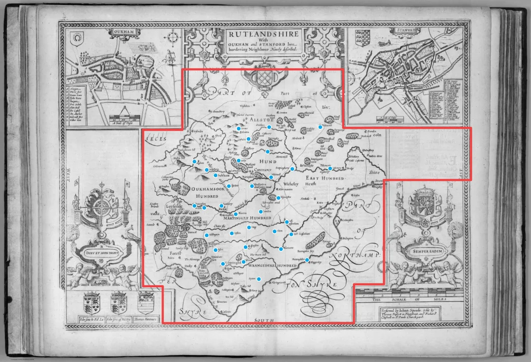
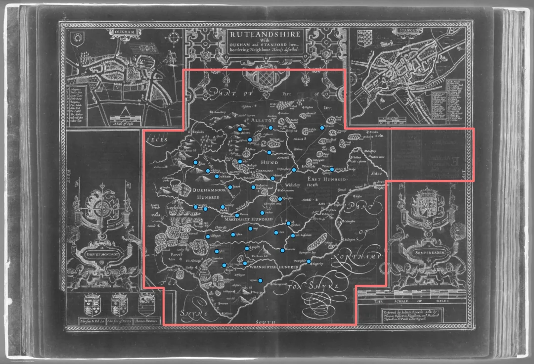
Separate map from decoration, match churches, read the scale

1. Separate the map from the decoration

Speed's sheet is a page of an atlas. The county map shares it with plans of Oakham and Stamford, a title cartouche, two coats of arms, a compass rose and a scale of miles — all drawn at a different scale or at none. A transformation fitted to the villages would place the Stamford town plan somewhere in Lincolnshire. Draw the outline of the map area in pixel coordinates once, by eye — MAP_AREA in the setup block below:

w, h = Image.open("data/speed_rutland.jpg").size
print(f"sheet {w} x {h} px; map area {Polygon(MAP_AREA).area / (w * h):.0%} of it")

sheet 12232 x 8343 px; map area 31% of it

2. Match church symbols to villages

Speed marks each parish with a small church and spells it his own way: Oukham, Vppingham, Edgeton, Lynden, Moorecote. The control point is the centre of the symbol, matched to OpenStreetMap's point for the modern village (POINTS, built in the setup block):

print(len(POINTS), "villages matched; missing:", missing or "none")

33 villages matched; missing: none

Some of Speed's villages cannot be matched at all. Martinsthorpe and Horn were already deserted or shrinking when he drew them and are farms or fields today; they are left out rather than guessed.

3. Read the scale bar

The scale of miles is a measurement Speed made, and it can be checked. The divisions are the only columns of the bar that are dark from top to bottom:

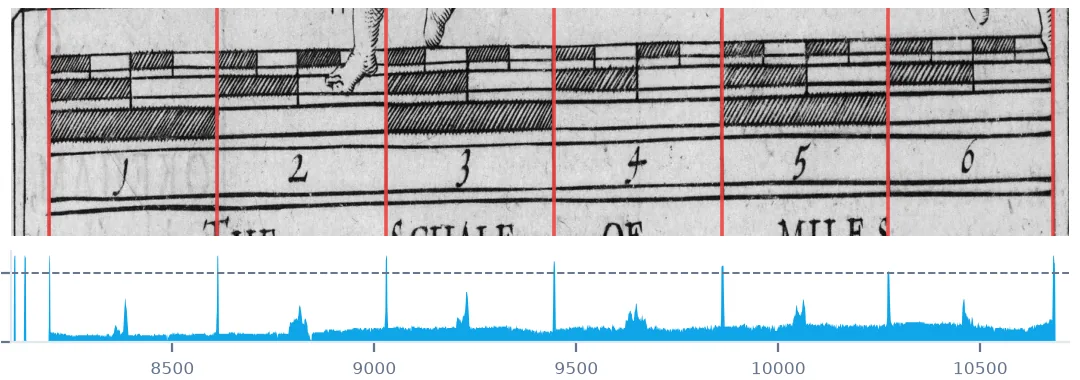
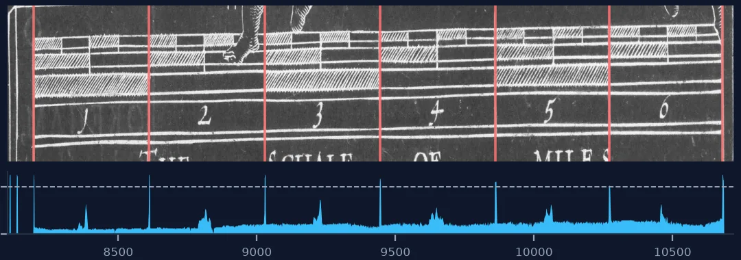
band = np.asarray(Image.open("data/speed_rutland.jpg").convert("L").crop((8100, 6800, 10700, 6860)), float)
cols = np.flatnonzero((band < 110).mean(axis=0) > 0.8) + 8100
divs = [g.mean() for g in np.split(cols, np.flatnonzero(np.diff(cols) > 3) + 1) if g.mean() > 8150]
px_per_mile = (divs[-1] - divs[0]) / (len(divs) - 1)
X = np.array([[1, c, r] for _, c, r, _, _ in POINTS], float)
A = np.linalg.lstsq(X, np.array([[e, n] for *_, e, n in POINTS]), rcond=None)[0]
m_per_px = np.hypot(*A[1])
print(f"{len(divs) - 1} miles over {divs[-1] - divs[0]:.0f} px: {px_per_mile:.1f} px per mile")
print(f"fitted {m_per_px:.2f} m per px, so Speed's mile is {px_per_mile * m_per_px:,.0f} m "
      f"({px_per_mile * m_per_px / 1609.344:.2f} statute miles)")

6 miles over 2486 px: 414.3 px per mile
fitted 4.80 m per px, so Speed's mile is 1,988 m (1.24 statute miles)

Speed's mile is about two kilometres, a quarter longer than the statute mile defined in 1593. Long "customary" miles were still common in Speed's time, and county maps used them; any distance read off the sheet in its own miles needs that factor.

4. Choose the transformation with leave-one-out

With 33 points, a polynomial has enough to work with. Score affine, polynomial 2 and a thin-plate spline the same way:

for label, opts in {"affine": ["METHOD=GCP_POLYNOMIAL", "MAX_GCP_ORDER=1"],
                    "polynomial 2": ["METHOD=GCP_POLYNOMIAL", "MAX_GCP_ORDER=2"],
                    "thin-plate spline": ["METHOD=GCP_TPS"]}.items():
    err = []
    for i, (k, c, r, e, n) in enumerate(POINTS):
        rest = POINTS[:i] + POINTS[i + 1:]
        v = gdal.Translate("", "data/speed_rutland.jpg", format="VRT", bandList=[1], outputSRS="EPSG:27700",
                           GCPs=[gdal.GCP(ee, nn, 0, cc, rr) for _, cc, rr, ee, nn in rest])
        x, y = gdal.Transformer(v, None, opts).TransformPoint(0, c, r)[1][:2]
        err.append(np.hypot(x - e, y - n))
    print(f"{label:18} leave-one-out RMS {np.sqrt(np.mean(np.square(err))):5.0f} m   worst {max(err):5.0f} m")

affine             leave-one-out RMS   695 m   worst  1423 m
polynomial 2       leave-one-out RMS   549 m   worst  1085 m
thin-plate spline  leave-one-out RMS   689 m   worst  1282 m

The opposite of the Victorian sheet: there, seven precise points favoured the spline and broke the polynomial; here, 33 imprecise ones favour the polynomial, which catches a smooth distortion across the county, while the spline gains almost nothing by bending to honour every village's individual error.

5. Warp, cut, and look

The quick answer warps with polynomial 2 at 10 m — Speed's linework is a pixel or two wide at about 4.8 m per pixel, so finer cells add nothing — and cuts to the map area. Then look at it with modern data:

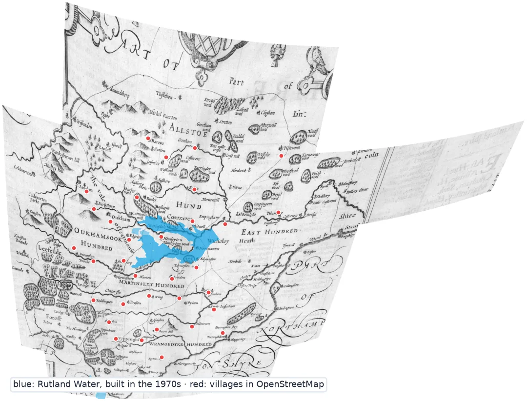
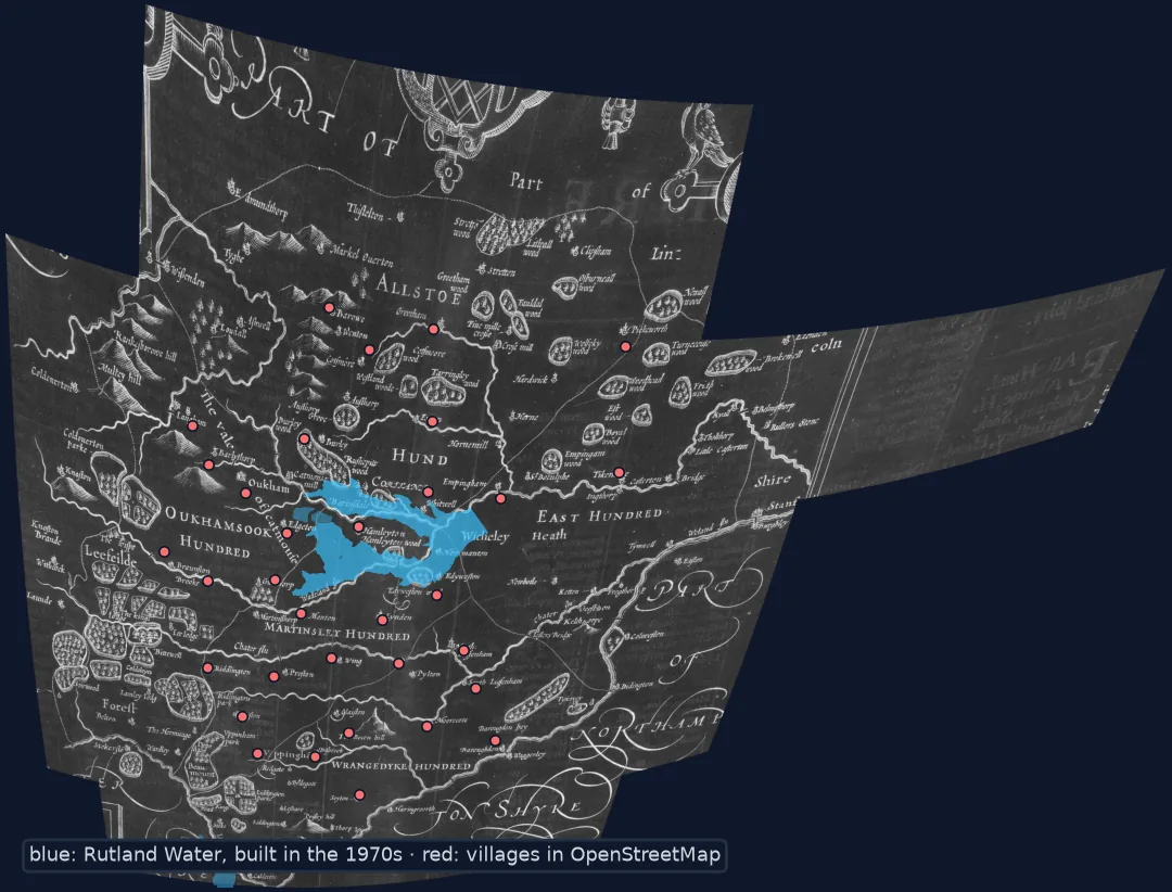
The warped sheet is curved at the edges. That is the polynomial extrapolating into the margins where there are no villages; the county itself, where the points are, is where the fit can be trusted.

Georeferencing Speed's Rutlandshire

The data used on this page

John Speed, Rutlandshire, 1676 Bassett & Chiswell edition of The Theatre of the Empire of Great Britaine (first published 1611–12), from the David Rumsey Map Collection, David Rumsey Map Center, Stanford Libraries, via Wikimedia Commons (public domain); OpenStreetMap from Geofabrik (1 January 2026; © OpenStreetMap contributors, ODbL). The church symbols were located by eye at full resolution.

from pathlib import Path

import geopandas as gpd
import numpy as np
import requests
from osgeo import gdal
from PIL import Image
from shapely.geometry import Polygon

gdal.UseExceptions()
Image.MAX_IMAGE_PIXELS = None            # 12,232 x 8,343 pixels
Path("data").mkdir(exist_ok=True)
UA = {"User-Agent": "spatialworkflow.io guide (https://www.spatialworkflow.io)"}
downloads = {
    "data/speed_rutland.jpg": "https://upload.wikimedia.org/wikipedia/commons/9/9c/Rutlandshire._%28insets%29_Oukham."
                              "_Stanford._%28IA_dr_rutlandshire-insets-oukham-stanford-12058072%29.jpg",
    "data/rutland.shp.zip": "https://download.geofabrik.de/europe/united-kingdom/england/rutland-260101-free.shp.zip",
}
for target, url in downloads.items():
    if not Path(target).exists():
        Path(target).write_bytes(requests.get(url, headers=UA, timeout=600).content)

SPEED_PX = {  # modern village name: (column, row) of Speed's church symbol
    "Oakham": (4960, 4035), "Langham": (4475, 3725), "Barleythorpe": (4755, 3920), "Egleton": (5265, 4290),
    "Braunston in Rutland": (4470, 4745), "Brooke": (4705, 4790), "Gunthorpe": (5095, 4745), "Manton": (5430, 4935),
    "Greetham": (6200, 2930), "Cottesmore": (5715, 3205), "Exton": (6165, 3500), "Empingham": (6730, 3890),
    "Whitwell": (6245, 4080), "Upper Hambleton": (5795, 4285), "Burley on the Hill": (5490, 3705), "Barrow": (5495, 2965),
    "Pickworth": (7375, 2930), "Tickencote": (7595, 3875), "Lyndon": (6005, 4880), "Edith Weston": (6415, 4555),
    "Wing": (5735, 5245), "Pilton": (6315, 5335), "North Luffenham": (6600, 5110), "South Luffenham": (6705, 5400),
    "Ridlington": (4755, 5425), "Preston": (5335, 5380), "Glaston": (5650, 5690), "Morcott": (6465, 5735),
    "Ayston": (4960, 5765), "Uppingham": (5125, 6080), "Bisbrooke": (5605, 6035), "Seaton": (5960, 6430),
    "Barrowden": (7070, 5985),
}

MAP_AREA = [(3300, 3000), (4200, 3000), (4200, 1600), (7900, 1600), (7900, 2950), (10850, 2950),
            (10850, 4150), (8850, 4150), (8850, 6550), (8150, 6550), (8150, 7450), (3750, 7450),
            (3750, 6600), (3300, 6600)]

places = gpd.read_file("/vsizip/data/rutland.shp.zip/gis_osm_places_free_1.shp").to_crs(27700)
places = places[places.fclass.isin(["village", "town", "hamlet"])].drop_duplicates("name").set_index("name")
missing = [k for k in SPEED_PX if k not in places.index]
POINTS = [(k, c, r, places.loc[k].geometry.x, places.loc[k].geometry.y) for k, (c, r) in SPEED_PX.items()]

def densify(ring, step=50):
    """Points every `step` pixels along a closed ring, so a curved warp can follow it."""
    ring = list(ring) + [ring[0]]
    out = []
    for (x0, y0), (x1, y1) in zip(ring[:-1], ring[1:]):
        k = max(1, int(np.hypot(x1 - x0, y1 - y0) // step))
        out += [(x0 + (x1 - x0) * i / k, y0 + (y1 - y0) * i / k) for i in range(k)]
    return out

print({p.name: f"{p.stat().st_size / 1e6:.1f} MB" for p in Path("data").iterdir() if p.suffix in (".jpg", ".zip")})

{'speed_rutland.jpg': '27.8 MB', 'rutland.shp.zip': '2.7 MB'}

Example 1: what happens without the cutline

Warp the whole sheet with the same transformation and the inset plans, arms and page margins come along, bent by a polynomial that was never fitted to them:

whole = gdal.Warp("", vrt, format="MEM", dstSRS="EPSG:27700", polynomialOrder=2, xRes=10, yRes=10, dstAlpha=True)
cutf = gdal.Open("data/speed_rutland_bng.tif")
for label, ds in (("whole sheet", whole), ("map area only", cutf)):
    gt = ds.GetGeoTransform()
    print(f"{label:14} {ds.RasterXSize * gt[1] / 1000:5.1f} km x {ds.RasterYSize * -gt[5] / 1000:5.1f} km")

whole sheet     75.7 km x  58.2 km
map area only   40.1 km x  30.6 km

The whole-sheet warp covers far more ground than the county, most of it the book's binding and margins pretending to be Leicestershire and Lincolnshire. With a polynomial, the further out a pixel is from the villages, the stranger its position; the cutline keeps only the part the points describe.

Example 2: the villages Speed placed worst

The leave-one-out errors of the polynomial fit, largest first, show where his map is least reliable:

v = gdal.Translate("", "data/speed_rutland.jpg", format="VRT", bandList=[1], outputSRS="EPSG:27700",
                   GCPs=[gdal.GCP(e, n, 0, c, r) for _, c, r, e, n in POINTS])
worst = []
for i, (k, c, r, e, n) in enumerate(POINTS):
    rest = POINTS[:i] + POINTS[i + 1:]
    vi = gdal.Translate("", "data/speed_rutland.jpg", format="VRT", bandList=[1], outputSRS="EPSG:27700",
                        GCPs=[gdal.GCP(ee, nn, 0, cc, rr) for _, cc, rr, ee, nn in rest])
    x, y = gdal.Transformer(vi, None, ["METHOD=GCP_POLYNOMIAL", "MAX_GCP_ORDER=2"]).TransformPoint(0, c, r)[1][:2]
    worst.append((round(float(np.hypot(x - e, y - n))), k, round(np.degrees(np.arctan2(x - e, y - n)))))
for d, k, bearing in sorted(worst, reverse=True)[:5]:
    print(f"{k:16} {d:5} m, displaced towards bearing {bearing % 360:3} deg")

Glaston           1085 m, displaced towards bearing 306 deg
Langham           1067 m, displaced towards bearing 305 deg
Braunston in Rutland   971 m, displaced towards bearing 149 deg
Pilton             804 m, displaced towards bearing 131 deg
Tickencote         752 m, displaced towards bearing 151 deg

These are the places to check before reading anything off Speed's map: a symbol a kilometre from its village is either a mistake in the map or a place that has moved, and the map alone cannot tell you which.

Early county maps against surveyed ones

The difference between an early county map and a modern survey is not just size of error; it is the kind of error. Speed compiled his maps from earlier ones — Christopher Saxton's county surveys of the 1570s among them — and from information gathered on journeys, with villages placed by direction and travelled distance. Errors in that process accumulate along routes and differ from parish to parish. A fit through the villages averages them; nothing removes them.

That shapes every choice on this page. Control points have to be features that existed in 1611 and still exist, which leaves churches and villages; there are not enough precise points to test a fine fit, but there are many rough ones. A smooth polynomial with 33 points can pick up the distortion common to a whole region of the county, while a spline would bend to each village's own mistake and gain almost nothing. And the result is good to about half a kilometre, so it should be used for questions at that scale: which parishes, which woods, which roads existed — not where a hedge ran.

The cutline matters for the same reason. A transformation is a statement about the area its control points cover. The inset plan of Stamford is drawn at a scale of its own; warping it with the county's transformation produces a confident-looking picture of nothing.

Reused plates, changed names and deserted villages

• Later editions reuse the plates. A 1676 printing shows the 1611 geography; date the content, not the paper.
• Names change. Match Speed's spellings by hand; a fuzzy matcher will happily pair Barowe with Barrowden.
• Deserted villages have no modern point; leave them out.
• Village points are fuzzy in OpenStreetMap; at Speed's accuracy that is fine, at the OS sheet's it is not.
• Speed's mile is about 2 km; convert before quoting distances.
• Rutland Water did not exist: the 1970s reservoir drowned the valley below Hambleton and the village of Nether Hambleton, so expect the old map to show a valley where today's data shows a lake.

Internal links

• How accurate is a historical map? — Speed against the OS six-inch sheet
• Georeferencing transformations explained — why 33 points change the choice
• How to download scanned historical maps — finding sheets on Wikimedia Commons
• Old map projections explained — what grid, if any, an early map was drawn on
• Old map is offset from modern data — telling the map's error from yours

FAQ

Can you georeference a 17th-century map?

Yes, with church or village symbols as control points. Expect an accuracy of hundreds of metres: Speed's Rutland fits to about 550 m (leave-one-out RMS) with a second-order polynomial.

Which transformation suits an early county map?

Test them. With many imprecise points, a second-order polynomial often predicts best, because it captures smooth distortion across the county without bending to individual errors.

How do I stop the decorations being warped?

Draw the map area as a polygon in pixel coordinates, push it through the same transformation into the target CRS, and pass it to gdal.Warp as a cutline with cropToCutline=True.

How long was a mile on old maps?

It varied. Measured against modern data, the mile on Speed's Rutland scale bar is about 2 km, a quarter longer than a statute mile.