
Ground Control Points Explained: What Makes a Good One
On this page
Problem statement
Every georeferenced map rests on its ground control points (GCPs): a handful of places identified on the scan and on the ground, asserted to be the same. The software will fit a transformation to any points you give it and report a tidy error figure. Whether the map then lands in the right place depends almost entirely on which points you chose and where they sit on the sheet — and that is easy to get wrong without noticing.
This page uses the seven control points picked on the Ordnance Survey six-inch sheet of Oakham (1884–1891) against OpenStreetMap to measure what matters: how many points, how spread out, and how to tell when one of them is lying.
Quick answer
A good control point is a feature that has not moved since the survey, can be located to a single point on both the map and the reference data, and sits where it helps — towards the edges of the sheet. Spread matters more than number:
subsets = []
for k in (3, 4):
    for sub in itertools.combinations(range(len(GCPS)), k):
        chosen = [GCPS[i] for i in sub]
        others = [g for i, g in enumerate(GCPS) if i not in sub]
        subsets.append(dict(k=k, names=[g[0] for g in chosen], hull=hull_share(chosen),
                            worst=max(errors(fit(chosen), others))))
df = pd.DataFrame(subsets)
print(df.sort_values("worst").iloc[[0, -1]][["k", "hull", "worst", "names"]].round(3).to_string(index=False))
k hull worst names
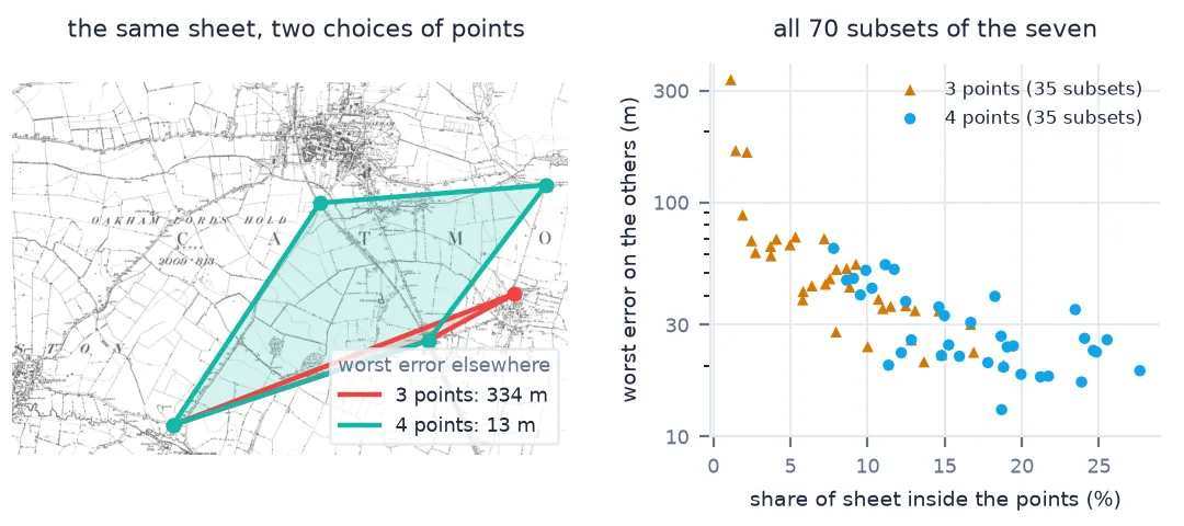
4 0.187 13.029 [brooke_rd_crossing, egleton_level_crossing, stamford_rd_guide_post, brooke_guide_post]
3 0.011 334.370 [egleton_church, egleton_level_crossing, brooke_guide_post]
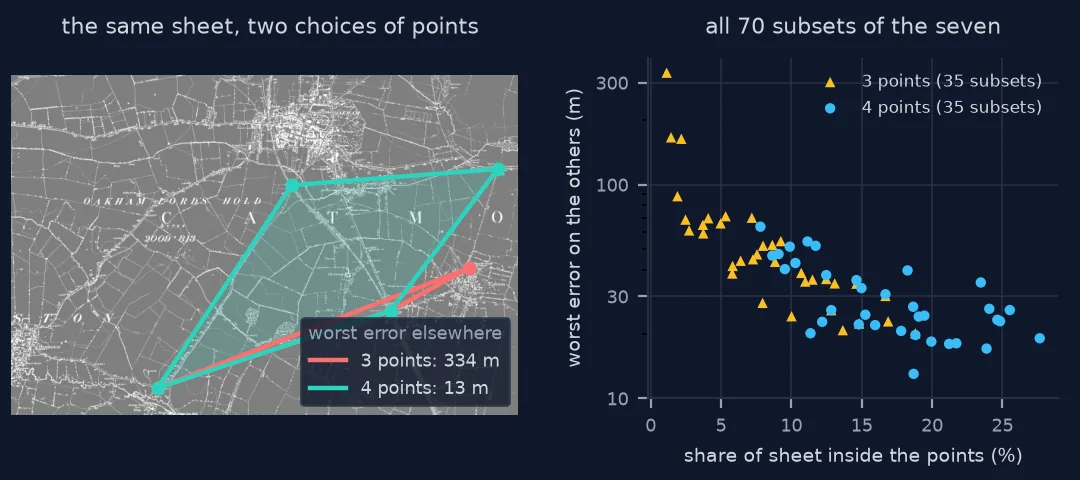
Three points crowded along one line put the rest of the sheet up to a third of a kilometre out. Four points that enclose a fifth of the sheet keep every other point within 13 m:
A pair and a claim, stable features, spread
1. A control point is a pair of coordinates and a claim
Each point has a position on the scan (column and row) and a position on the ground (here, easting and northing in British National Grid), plus a name so you can find it again:
for name, px, py, e, n in GCPS:
    print(f"{name:24} ({px:4}, {py:4}) <-> ({e:9.1f}, {n:9.1f})")
oakham_church (3141, 487) <-> ( 486065.6, 308906.1)
egleton_church (4824, 2031) <-> ( 487598.5, 307540.3)
brooke_rd_crossing (2956, 1159) <-> ( 485892.0, 308306.8)
egleton_level_crossing (3998, 2481) <-> ( 486838.1, 307119.0)
stamford_rd_guide_post (5127, 988) <-> ( 487872.3, 308486.1)
braunston_rd_bridleway (1263, 1675) <-> ( 484382.4, 307839.2)
brooke_guide_post (1547, 3292) <-> ( 484648.2, 306376.1)
The pair is a claim, not a measurement: "the block marked All Saints Church on the 1880s sheet is the building OpenStreetMap calls All Saints today". If the claim is false — the church was rebuilt on a new footprint, or the map's symbol is not where the building is — the transformation fits the error faithfully.
2. Choose features that have not moved
Over 130 years, some things on the six-inch sheet stayed put and many did not:
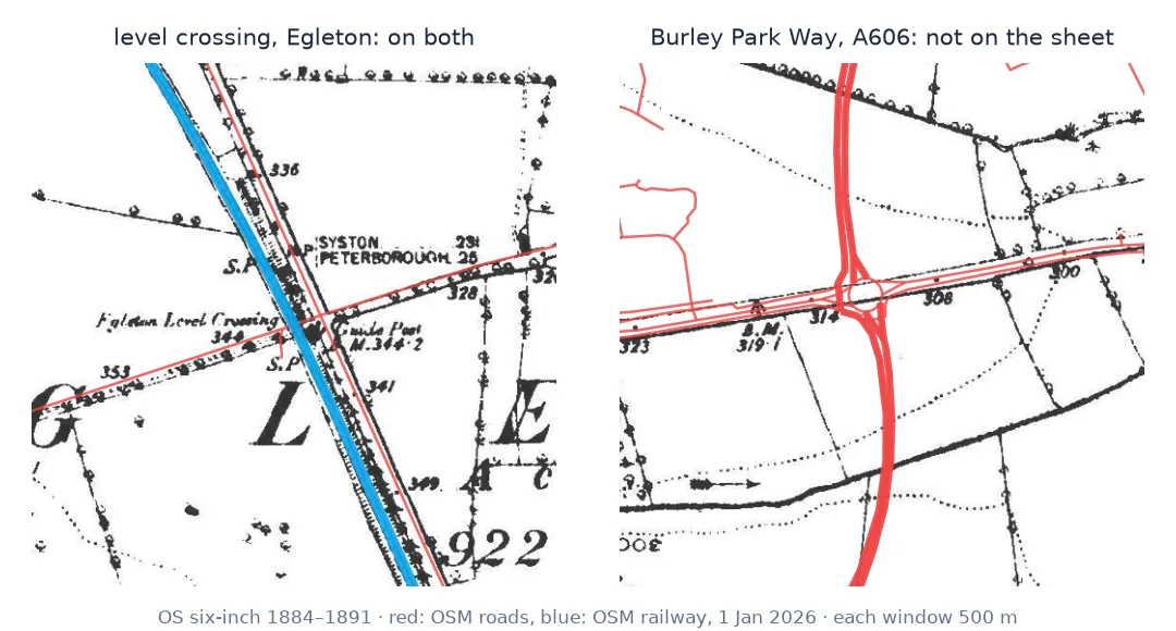
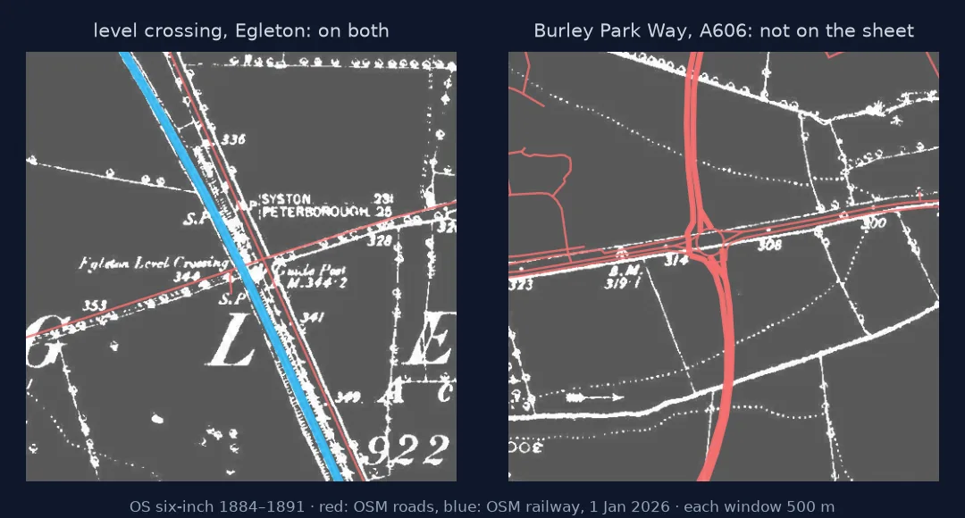
Churches, railway lines (Oakham's dates from 1848) and old road junctions in villages are the usual anchors. Field corners, footpaths and roads that have since been widened or straightened are not: they may be in the same place, but you cannot check it.
3. Spread them across the sheet
An affine transformation is a plane tilted through the points. Inside the points' convex hull it interpolates; outside it extrapolates, and small errors in the points swing into large errors at the far edges:
for k in (3, 4):
    d = df[df.k == k]
    print(f"{k} points: correlation of spread with worst error {d.hull.corr(d.worst, method='spearman'):+.2f}; "
          f"worst error ranges {d.worst.min():.0f}-{d.worst.max():.0f} m, median {d.worst.median():.0f} m")
3 points: correlation of spread with worst error -0.89; worst error ranges 20-334 m, median 44 m
4 points: correlation of spread with worst error -0.64; worst error ranges 13-64 m, median 26 m
The more of the sheet the points enclose, the smaller the worst error elsewhere. With three points the spread almost decides the result on its own.
4. Use more than the minimum
Three points determine an affine transformation exactly, which means there is nothing left over to check them with. Every point beyond the minimum is a check:
for k in range(3, 7):
    worst = [max(errors(fit([GCPS[i] for i in sub]), [g for i, g in enumerate(GCPS) if i not in sub]))
             for sub in itertools.combinations(range(7), k)]
    print(f"{k} points: median worst error {np.median(worst):5.1f} m over {len(worst)} subsets")
3 points: median worst error 44.1 m over 35 subsets
4 points: median worst error 25.9 m over 35 subsets
5 points: median worst error 20.5 m over 21 subsets
6 points: median worst error 16.9 m over 7 subsets
Going from three points to four cuts the typical worst error from 44 m to 26 m; after that the gains are smaller, but each extra point is another chance to catch a mistake.
5. Test each point against the others
With more than the minimum, leave each point out, fit the rest, and see how far it lands from where you said it was:
loo = {g[0]: errors(fit(GCPS[:i] + GCPS[i + 1:]), [g])[0] for i, g in enumerate(GCPS)}
print({k: round(v, 1) for k, v in sorted(loo.items(), key=lambda kv: kv[1])})
{'egleton_church': 8.5, 'brooke_rd_crossing': 14.6, 'oakham_church': 16.5, 'brooke_guide_post': 16.9, 'braunston_rd_bridleway': 18.4, 'stamford_rd_guide_post': 21.8, 'egleton_level_crossing': 22.2}
No point stands out on this sheet, which is what a good set looks like: every error sits within a factor of three of every other. A point twice as bad as the next worst deserves a second look at the scan.
One bad point among seven good ones
The data used on this page
The seven control points picked on the Ordnance Survey six-inch sheet Rutland 009-NW (1884–1891, Wikimedia Commons, public domain) against OpenStreetMap (Geofabrik, 1 January 2026; © OpenStreetMap contributors, ODbL), as in the control-point guide. Only the points and the sheet's pixel size are needed.
import itertools

import numpy as np
import pandas as pd
from scipy.spatial import ConvexHull

SHEET_W, SHEET_H = 5343, 3573          # pixels, Rutland 009-NW
GCPS = [  # (id, pixel, line, easting, northing)
    ("oakham_church",          3141,  487, 486065.6, 308906.1),
    ("egleton_church",         4824, 2031, 487598.5, 307540.3),
    ("brooke_rd_crossing",     2956, 1159, 485892.0, 308306.8),
    ("egleton_level_crossing", 3998, 2481, 486838.1, 307119.0),
    ("stamford_rd_guide_post", 5127,  988, 487872.3, 308486.1),
    ("braunston_rd_bridleway", 1263, 1675, 484382.4, 307839.2),
    ("brooke_guide_post",      1547, 3292, 484648.2, 306376.1),
]

def fit(points):
    """Affine pixel -> British National Grid, least squares."""
    A = np.array([[g[1], g[2], 1] for g in points], float)
    return (np.linalg.lstsq(A, [g[3] for g in points], rcond=None)[0],
            np.linalg.lstsq(A, [g[4] for g in points], rcond=None)[0])

def errors(coef, points):
    cx, cy = coef
    return [float(np.hypot(cx @ (px, py, 1) - e, cy @ (px, py, 1) - n)) for _, px, py, e, n in points]

def hull_share(points):
    return ConvexHull(np.array([[g[1], g[2]] for g in points], float)).volume / (SHEET_W * SHEET_H)

print(len(GCPS), "control points")
7 control points
Example 1: one bad point among good ones
Shift one point by 60 pixels — about 54 m, an easy slip at the scale you click at — and run the leave-one-out test again:
bad = list(GCPS)
name, px, py, e, n = bad[4]
bad[4] = (name, px - 60, py, e, n)
loo_bad = {g[0]: errors(fit(bad[:i] + bad[i + 1:]), [g])[0] for i, g in enumerate(bad)}
for k, v in sorted(loo_bad.items(), key=lambda kv: -kv[1])[:3]:
    print(f"{k:24} {v:6.1f} m   (was {loo[k]:5.1f})")
stamford_rd_guide_post 72.9 m (was 21.8)
brooke_guide_post 46.8 m (was 16.9)
egleton_level_crossing 35.5 m (was 22.2)
The moved point rises to the top of the list. Leave-one-out finds a bad point because the others, fitted without it, disagree with it; residuals from a fit that includes it would spread the error over all seven.
Example 2: how a point's position changes its influence
A point at the edge of the sheet pulls harder on the fit than one in the middle. Leverage, from the hat matrix of the least-squares fit, measures that pull:
A = np.array([[g[1], g[2], 1] for g in GCPS], float)
leverage = np.diag(A @ np.linalg.inv(A.T @ A) @ A.T)
print(pd.Series(leverage, index=[g[0] for g in GCPS]).round(2).sort_values(ascending=False).to_string())
brooke_guide_post 0.66
braunston_rd_bridleway 0.48
oakham_church 0.46
stamford_rd_guide_post 0.43
egleton_church 0.39
egleton_level_crossing 0.34
brooke_rd_crossing 0.23
Leverage runs from 0 to 1; with 3 coefficients and 7 points it averages 3/7 = 0.43. Brooke guide post, alone in the south-west corner, has the most; Brooke Road crossing, in the middle of the cloud, the least. The points that make the spread carry the fit, which is exactly why an error in one of them costs the most. Spend your care where the leverage is.
Points constrain and test the fit
A control point does two jobs. It constrains the transformation, pinning one place on the scan to one place on the ground, and — if there are more points than the transformation needs — it checks the others. The first job wants points at the edges, where they control the extrapolation. The second wants more points than the minimum, so that each can be tested against a fit it did not influence.
The deeper difficulty is that a control point joins two different representations of the world. The 1880s surveyor drew a church as a solid block at its true footprint; OpenStreetMap draws it as a polygon digitised from aerial imagery. A level crossing is a line crossing a line in both — that is why crossings are good points: the intersection is defined the same way on both sides. A road junction in a town may have been realigned twice. A field corner is only as good as the hedge, which may have been grubbed out in the 1960s and replanted a few metres away.
So "unchanged" is a historical judgement, not a geometric one, and the only test the data offers is consistency: if a point disagrees with the rest by much more than they disagree with each other, either it moved, or you clicked it wrong, or the map was wrong there. Leave-one-out cannot say which — only that one of those happened.
Unchecked fits, collinearity and edge leverage
- Three points cannot be checked. An affine fit through three points has zero residual and no redundancy.
- Near-collinear points are almost as bad as two points: they leave the direction across the line unconstrained.
- Edge points carry the most leverage; check them twice.
- Name every point. A list of anonymous coordinates cannot be re-checked later.
- Record the reference data and its date — OpenStreetMap on 1 January 2026 here — because the reference changes too.
- Corners of the sheet are often blank countryside; a lone farmhouse or a parish boundary stone may be the only option.
Internal links
- How to pick ground control points for a scanned map — the practical procedure for these seven
- Georeferencing explained — where control points fit in the whole process
- Georeferencing transformations explained — how many points each method needs
- Low GCP residuals, but the map is still wrong — when the error table lies
- How accurate is a historical map? — the error you cannot remove
FAQ
What is a ground control point?
A location identified both on an image and on the ground (or in reference data with known coordinates). A set of them is what a georeferencing transformation is fitted to.
How many ground control points do I need?
Three is the minimum for an affine fit; use at least four to six so each can be checked against the rest. On the Oakham sheet the median worst error fell from 44 m with three points to 26 m with four.
Where should I put control points?
Spread across the sheet, especially towards the edges and corners. Points clustered in one area leave the rest of the map to extrapolation.
What makes a feature a good control point?
It existed when the map was made and still exists, it is unchanged in position, and it can be located to one point in the same way on both sources — a church, a railway crossing, an old junction.
How do I find a bad control point?
Leave each point out in turn, fit the others, and measure how far the omitted point lands from its stated position. The bad one stands out.