How to Draw a Distortion Grid on an Old Map in Python

Problem statement

A single accuracy figure — "700 m RMS" — says how wrong an old map is on average, but not where or how. Is one corner squeezed? Is a river valley stretched? Did the mapmaker turn the north of the county against the south? Historians of cartography answer that with a distortion grid: a regular grid of today's coordinates, drawn onto the old map through the same control points that georeference it. Where the map is accurate the grid stays square; where it is not, the grid bends, stretches and twists.

This page draws one on John Speed's Rutlandshire (1611, here in the 1676 edition) and on the Ordnance Survey six-inch sheet of Oakham (1884–1891), and turns the bent grid into numbers: how much bigger or smaller, and how much rotated, each square kilometre is on the old map.

Quick answer

Build lines of constant easting and northing in the modern CRS, and send them backwards through a GDAL transformer fitted to the control points — direction 1 is world to pixel — so they land on the scan:

vrt = gdal.Translate("", "data/speed_rutland.jpg", format="VRT", bandList=[1], outputSRS="EPSG:27700",
                     GCPs=[gdal.GCP(e, n, 0, c, r) for _, c, r, e, n in POINTS])
t = gdal.Transformer(vrt, None, ["METHOD=GCP_TPS"])
lines = []
for e in np.arange(483000, 500001, 1000):                      # 1 km eastings
    lines.append(np.array(t.TransformPoints(1, [(e, n, 0) for n in np.linspace(298000, 316000, 80)])[0])[:, :2])
for n in np.arange(298000, 316001, 1000):                      # 1 km northings
    lines.append(np.array(t.TransformPoints(1, [(e, n, 0) for e in np.linspace(483000, 500000, 80)])[0])[:, :2])
print(len(lines), "grid lines; first starts at pixel", np.round(lines[0][0]).astype(int))

37 grid lines; first starts at pixel [4431 6745]

Plot the lines over the scan. Speed's grid buckles; the Victorian sheet's stays square:

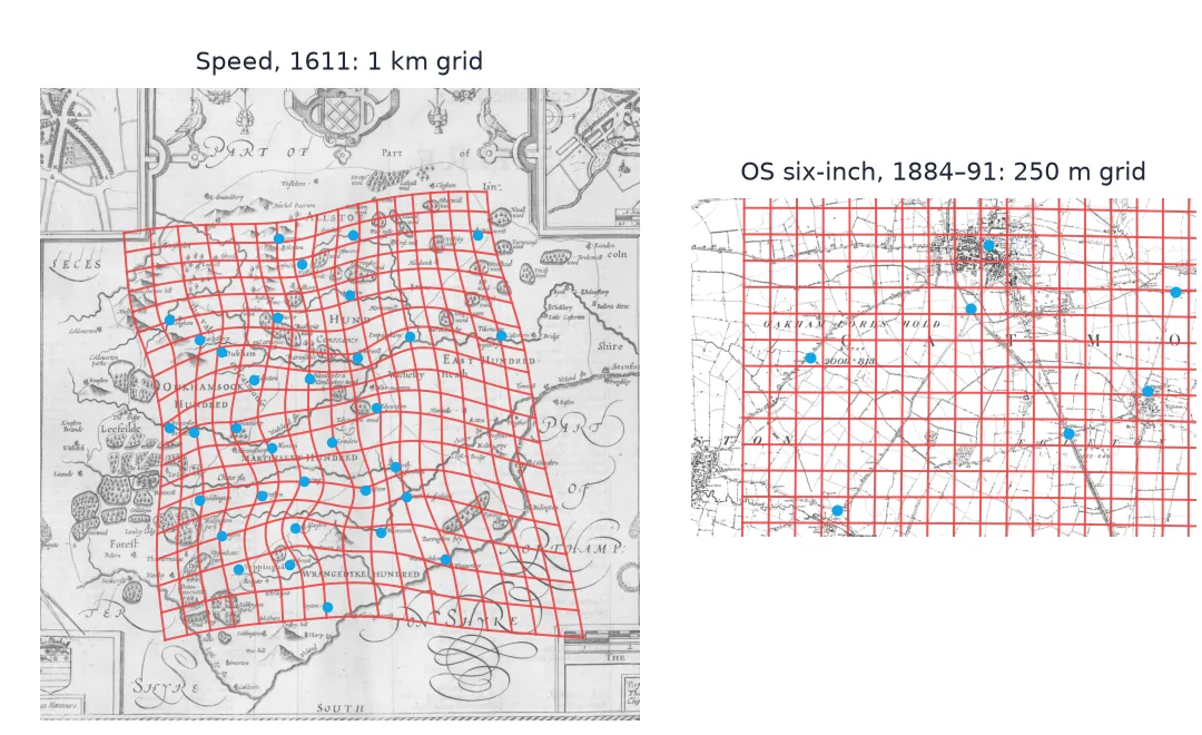
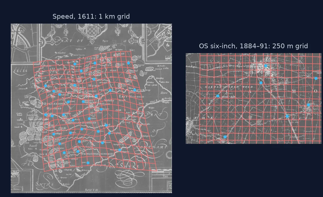
A local fit, a matching grid spacing, through the transform

1. Fit a transformation that follows local distortion

A distortion grid has to show local error, so it needs a transformation that passes through the control points rather than averaging them. A thin-plate spline does exactly that — at every village it is exact, and between villages it bends as little as possible. An affine fit would draw a perfectly regular grid on any map and show nothing. Near Oakham, the two disagree about the size of a square kilometre:

for label, opts in (("affine", ["METHOD=GCP_POLYNOMIAL", "MAX_GCP_ORDER=1"]), ("spline", ["METHOD=GCP_TPS"])):
    tt = gdal.Transformer(vrt, None, opts)
    corners = np.array(tt.TransformPoints(1, [(486000, 308000, 0), (487000, 308000, 0), (486000, 309000, 0)])[0])[:, :2]
    print(f"{label:7} 1 km east is {np.hypot(*(corners[1] - corners[0])):5.1f} px, 1 km north is {np.hypot(*(corners[2] - corners[0])):5.1f} px")

affine  1 km east is 205.8 px, 1 km north is 206.7 px
spline  1 km east is 230.8 px, 1 km north is 221.2 px

2. Choose a grid spacing that matches the map

Grid lines should be several times further apart than the map's error, or every cell is noise. Speed's error is several hundred metres, so 1 km; the six-inch sheet's is about 20 m, so 250 m shows plenty of cells without crowding.

3. Send the grid through the transformer backwards

TransformPoints(1, ...) asks the transformer for the inverse — world to pixel. Densify each line (80 points here) so its curve shows. Restrict the grid to roughly the area the control points cover: outside it, a spline shows nothing but its own extrapolation.

4. Measure each cell

The four corners of each grid square land somewhere on the scan. The area of that quadrilateral, relative to the typical cell, is how much the old map enlarged or shrank that square kilometre; the direction of its southern edge is how much it turned it:

ratio, rot, inside = cell_stats(POINTS, 1000)
print(f"{inside.sum()} cells inside the villages' hull")
print(f"area on the map vs typical: 5th-95th percentile {np.percentile(ratio[inside], 5):.2f}x to {np.percentile(ratio[inside], 95):.2f}x")
print(f"rotation vs typical:        5th-95th percentile {np.percentile(rot[inside], 5):+.1f} to {np.percentile(rot[inside], 95):+.1f} deg")

192 cells inside the villages' hull
area on the map vs typical: 5th-95th percentile 0.65x to 1.54x
rotation vs typical:        5th-95th percentile -16.7 to +19.7 deg

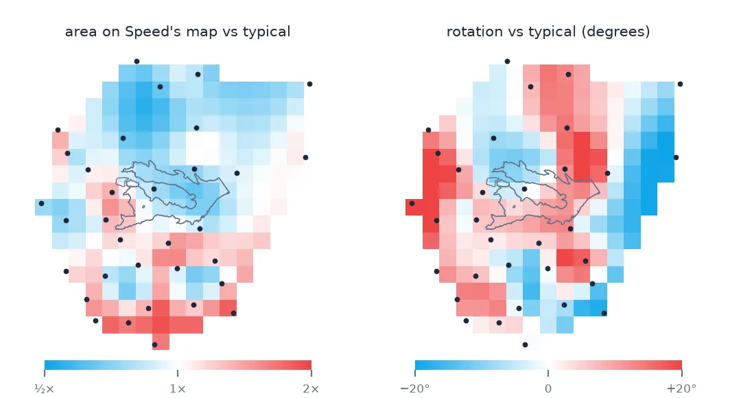
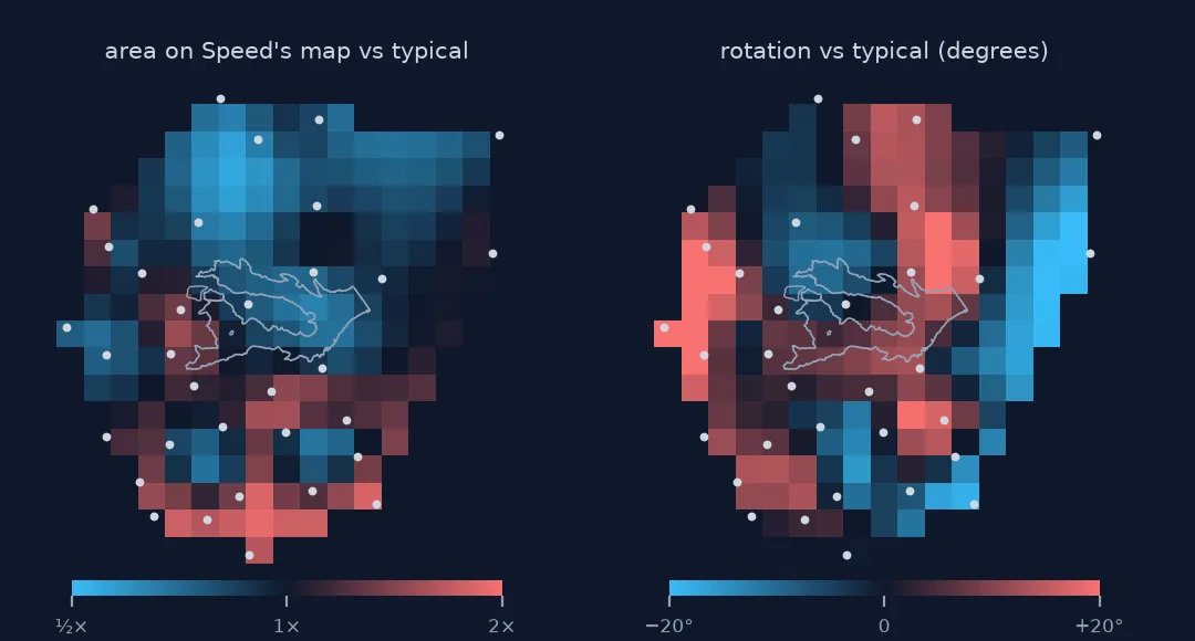
Some square kilometres are drawn at two-thirds of their typical size and some at half again; the drawing turns by up to twenty degrees either way from one part of the county to the next. Those are the parts of Speed's map where village positions were estimated from each other along routes rather than fixed, and they are the map's real structure of error.

5. Compare with a map you trust

The same procedure on the OS sheet is the control experiment:

os_ratio, os_rot, os_inside = cell_stats(OS, 250, scan="data/os_009-NW.jpg")
print(f"OS sheet: area 5th-95th {np.percentile(os_ratio[os_inside], 5):.2f}x-{np.percentile(os_ratio[os_inside], 95):.2f}x, "
      f"rotation {np.percentile(os_rot[os_inside], 5):+.1f} to {np.percentile(os_rot[os_inside], 95):+.1f} deg")

OS sheet: area 5th-95th 0.98x-1.01x, rotation -0.8 to +0.1 deg

A map that was surveyed rather than compiled gives an almost uniform grid. That contrast — not either grid alone — is what a distortion grid is for.

Drawing a grid over Speed's map

The data used on this page

John Speed, Rutlandshire, 1676 Bassett & Chiswell edition (first published 1611–12), from the David Rumsey Map Collection, David Rumsey Map Center, Stanford Libraries, via Wikimedia Commons (public domain); the Ordnance Survey six-inch sheet Rutland 009-NW (1884–1891, Wikimedia Commons, public domain); OpenStreetMap from Geofabrik (1 January 2026; © OpenStreetMap contributors, ODbL). The control points are those of the early county map guide and the control-point guide.

from pathlib import Path

import geopandas as gpd
import numpy as np
import requests
from osgeo import gdal
from PIL import Image
from shapely.geometry import MultiPoint, Point

gdal.UseExceptions()
Image.MAX_IMAGE_PIXELS = None
Path("data").mkdir(exist_ok=True)
UA = {"User-Agent": "spatialworkflow.io guide (https://www.spatialworkflow.io)"}
downloads = {
    "data/speed_rutland.jpg": "https://upload.wikimedia.org/wikipedia/commons/9/9c/Rutlandshire._%28insets%29_Oukham."
                              "_Stanford._%28IA_dr_rutlandshire-insets-oukham-stanford-12058072%29.jpg",
    "data/os_009-NW.jpg": "https://upload.wikimedia.org/wikipedia/commons/a/a0/"
                          "Map_of_Rutland_OS_Map_name_009-NW%2C_Ordnance_Survey%2C_1884-1891.jpg",
    "data/rutland.shp.zip": "https://download.geofabrik.de/europe/united-kingdom/england/rutland-260101-free.shp.zip",
}
for target, url in downloads.items():
    if not Path(target).exists():
        Path(target).write_bytes(requests.get(url, headers=UA, timeout=600).content)

SPEED_PX = {  # modern village name: (column, row) of Speed's church symbol
    "Oakham": (4960, 4035), "Langham": (4475, 3725), "Barleythorpe": (4755, 3920), "Egleton": (5265, 4290),
    "Braunston in Rutland": (4470, 4745), "Brooke": (4705, 4790), "Gunthorpe": (5095, 4745), "Manton": (5430, 4935),
    "Greetham": (6200, 2930), "Cottesmore": (5715, 3205), "Exton": (6165, 3500), "Empingham": (6730, 3890),
    "Whitwell": (6245, 4080), "Upper Hambleton": (5795, 4285), "Burley on the Hill": (5490, 3705), "Barrow": (5495, 2965),
    "Pickworth": (7375, 2930), "Tickencote": (7595, 3875), "Lyndon": (6005, 4880), "Edith Weston": (6415, 4555),
    "Wing": (5735, 5245), "Pilton": (6315, 5335), "North Luffenham": (6600, 5110), "South Luffenham": (6705, 5400),
    "Ridlington": (4755, 5425), "Preston": (5335, 5380), "Glaston": (5650, 5690), "Morcott": (6465, 5735),
    "Ayston": (4960, 5765), "Uppingham": (5125, 6080), "Bisbrooke": (5605, 6035), "Seaton": (5960, 6430),
    "Barrowden": (7070, 5985),
}
places = gpd.read_file("/vsizip/data/rutland.shp.zip/gis_osm_places_free_1.shp").to_crs(27700)
places = places[places.fclass.isin(["village", "town", "hamlet"])].drop_duplicates("name").set_index("name")
POINTS = [(k, c, r, places.loc[k].geometry.x, places.loc[k].geometry.y) for k, (c, r) in SPEED_PX.items()]
OS = [  # (id, pixel, line, easting, northing) on six-inch sheet 009-NW
    ("oakham_church",          3141,  487, 486065.6, 308906.1),
    ("egleton_church",         4824, 2031, 487598.5, 307540.3),
    ("brooke_rd_crossing",     2956, 1159, 485892.0, 308306.8),
    ("egleton_level_crossing", 3998, 2481, 486838.1, 307119.0),
    ("stamford_rd_guide_post", 5127,  988, 487872.3, 308486.1),
    ("braunston_rd_bridleway", 1263, 1675, 484382.4, 307839.2),
    ("brooke_guide_post",      1547, 3292, 484648.2, 306376.1),
]

def cell_stats(points, spacing, scan="data/speed_rutland.jpg"):
    """Area (relative to the median cell) and rotation (degrees from the median) of every grid cell on
    the scan, through a thin-plate spline; `inside` marks cells whose centre is inside the points' hull."""
    v = gdal.Translate("", scan, format="VRT", bandList=[1], outputSRS="EPSG:27700",
                       GCPs=[gdal.GCP(e, n, 0, c, r) for _, c, r, e, n in points])
    tt = gdal.Transformer(v, None, ["METHOD=GCP_TPS"])
    E = np.array([g[3] for g in points]); N = np.array([g[4] for g in points])
    es = np.arange(np.floor(E.min() / spacing) * spacing, np.ceil(E.max() / spacing) * spacing + 1, spacing)
    ns = np.arange(np.floor(N.min() / spacing) * spacing, np.ceil(N.max() / spacing) * spacing + 1, spacing)
    ge, gn = np.meshgrid(es, ns)
    px = np.array(tt.TransformPoints(1, [(e, n, 0) for e, n in zip(ge.ravel(), gn.ravel())])[0])[:, :2]
    px = px.reshape(len(ns), len(es), 2)
    a, b, c, d = px[:-1, :-1], px[:-1, 1:], px[1:, :-1], px[1:, 1:]
    cross = lambda p, q: p[..., 0] * q[..., 1] - q[..., 0] * p[..., 1]
    area = 0.5 * np.abs(cross(a, b) + cross(b, d) + cross(d, c) + cross(c, a))
    rot = np.degrees(np.arctan2(-(b[..., 1] - a[..., 1]), b[..., 0] - a[..., 0]))
    hull = MultiPoint([(g[3], g[4]) for g in points]).convex_hull
    inside = np.array([[hull.contains(Point(x + spacing / 2, y + spacing / 2)) for x in es[:-1]] for y in ns[:-1]])
    return area / np.median(area), rot - np.median(rot), inside

print(len(POINTS), "Speed points,", len(OS), "OS points")

33 Speed points, 7 OS points

Example 1: draw the grid and save it

The quick answer's lines, plotted over a reduced copy of the scan, are the figure at the top of this page:

import matplotlib
matplotlib.use("Agg")
import matplotlib.pyplot as plt

x0, y0, x1, y1 = 3250, 1550, 8900, 7500
img = np.asarray(Image.open("data/speed_rutland.jpg").convert("L").crop((x0, y0, x1, y1)).reduce(5))
fig, ax = plt.subplots(figsize=(6, 6.3), dpi=150)
ax.imshow(img, cmap="gray", extent=(x0, x1, y1, y0))
for L in lines:
    ax.plot(L[:, 0], L[:, 1], color="#ef4444", lw=0.7)
ax.plot([p[1] for p in POINTS], [p[2] for p in POINTS], "o", ms=3, color="#0ea5e9")
ax.set_xlim(x0, x1); ax.set_ylim(y1, y0); ax.set_axis_off()
fig.savefig("data/speed_distortion_grid.png", bbox_inches="tight")
print(Path("data/speed_distortion_grid.png").stat().st_size > 100_000)

True

Example 2: which way is "north" on Speed's map?

The median rotation of the grid is Speed's overall orientation against the National Grid — the same thing the affine fit's rotation measures:

v = gdal.Translate("", "data/speed_rutland.jpg", format="VRT", bandList=[1], outputSRS="EPSG:27700",
                   GCPs=[gdal.GCP(e, n, 0, c, r) for _, c, r, e, n in POINTS])
tt = gdal.Transformer(v, None, ["METHOD=GCP_TPS"])
p = np.array(tt.TransformPoints(1, [(490000, 305000, 0), (490000, 315000, 0)])[0])[:, :2]
bearing = np.degrees(np.arctan2(p[1, 0] - p[0, 0], -(p[1, 1] - p[0, 1])))
print(f"grid north on Speed's sheet points {bearing:+.1f} deg from the top of the page")

grid north on Speed's sheet points -4.6 deg from the top of the page

A few degrees, consistent with the affine fit's four. The page's "North" is close to grid north overall; the twenty-degree local twists in the rotation map are where individual parts of the county are turned against each other.

Reversing the usual direction of a warp

A distortion grid reverses the usual direction of georeferencing. Normally the old map is warped to fit a modern grid, and the distortion disappears into the resampling. Drawing the modern grid onto the old map leaves the old map untouched and puts the distortion on display, in the map's own space, where a historian can relate it to what the map shows: a river the mapmaker followed, a road he travelled, a part of the county he did not visit.

The grid is only as meaningful as the control points. Between points, a thin-plate spline bends as smoothly as it can, so a cell's shape is an interpolation of the errors at the villages around it; one misidentified village bends every cell near it. That is why the grid should be confined to the points' hull, why the grid spacing should be larger than the map's error, and why the cell statistics on this page are percentiles rather than extremes. A few cells at two or three times their size usually mean one bad point, not a strange map.

The OS comparison is not a formality. Without it, a grid that bends by ten per cent could be read as the map's distortion when it is the noise in your control points. With a precise map treated the same way alongside, the difference between the two grids is the difference between the maps.

Splines, hulls and spacing against error

• Use a spline, not affine, for the grid; an affine grid is always perfectly regular.
• Stay inside the points' hull. Outside it the grid shows the spline's extrapolation, not the map.
• Spacing larger than the error. At 200 m on Speed's map every cell is noise.
• Check outliers first. One wrong control point makes a local knot in the grid; fix the point before interpreting the knot.
• Inverse transforms of splines are iterative in GDAL; very coarse densification can miss sharp bends.
• Rotation angles on the scan are measured with rows increasing downwards; flip the sign of the row difference.

Internal links

• How accurate is a historical map? — the single-number version of this
• How to georeference an early county map — the Speed control points
• Georeferencing transformations explained — what the spline is doing
• Warped map is folded or stretched — when the grid folds over itself
• Ground control points explained — keeping the grid's input honest

FAQ

What is a distortion grid?

A regular grid of modern coordinates drawn onto an old map through the transformation that links them. Where the old map is accurate the grid stays regular; where it is distorted the grid bends.

How do I make a distortion grid in Python?

Fit a GDAL transformer (preferably a thin-plate spline) to the control points, build densified lines of constant easting and northing, and transform them with TransformPoints(1, ...) — the inverse, world to pixel — then plot them over the scan.

Is this what MapAnalyst does?

The idea is the same; MapAnalyst offers several interpolation methods and its own visualisations. The GDAL route here keeps the grid in the same pipeline as the georeferencing.

How distorted is John Speed's map of Rutland?

Locally, quite a lot: between the 5th and 95th percentiles, square kilometres are drawn from 0.65 to 1.54 times their typical size and turned by about ±20 degrees, while the overall orientation is within a few degrees of grid north.