
How to Digitise Features from an Old Map in Python
On this page
Problem statement
A georeferenced old map is still a picture: to measure anything on it — how much woodland a parish had, how long its roads were — the features have to become polygons and lines with coordinates. Tracing by hand in QGIS is accurate and slow. Thresholding the scan is fast and, on a black-and-white Ordnance Survey sheet, nearly useless: buildings, lettering, hedgerow trees, field boundaries and woodland symbols are all the same black.
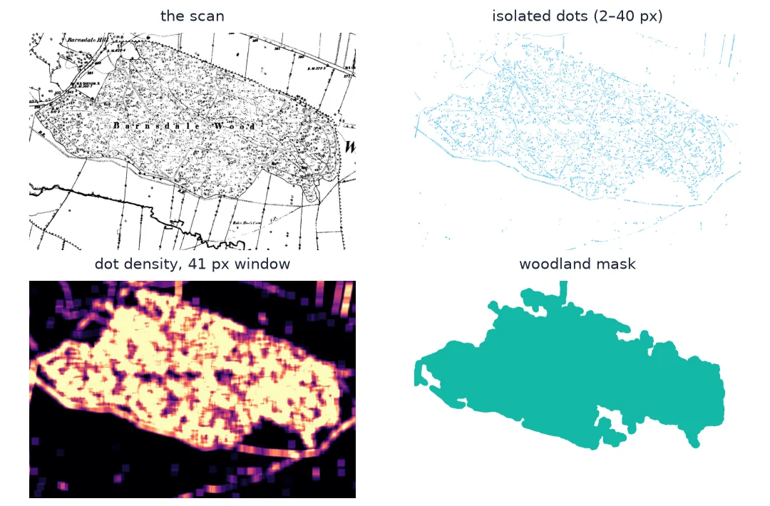
The way through is to look for what makes a feature different on the map, not what makes it dark. On the six-inch sheets, woodland is drawn as a dense stipple of small tree symbols, and nothing else on the sheet looks like that. This page turns that texture into woodland polygons for Rutland sheet 009-NE (surveyed 1884–1891), georeferences them, and checks how sensitive the result is to the choices made along the way.
Quick answer
Find the small, isolated ink marks, measure how densely they occur, threshold the density, and keep only regions thick enough to be woods:
im = np.asarray(Image.open("data/os_009-NE.jpg").convert("L"))
lab, _ = ndi.label(im < 128)
sizes = np.bincount(lab.ravel())
is_dot = (sizes >= 2) & (sizes <= 40)
is_dot[0] = False
density = ndi.uniform_filter(is_dot[lab].astype(float), size=41)          # share of dot pixels nearby
mask = ndi.binary_fill_holes(ndi.binary_opening(density > 0.04, structure=DISK15))
L, k = ndi.label(mask)
thick = np.r_[False, ndi.maximum(ndi.distance_transform_edt(mask), L, range(1, k + 1)) >= 35]
mask = thick[L]
woods = to_polygons(mask, "009-NE")
print(len(woods), "woods,", round(woods.area.sum() / 1e4, 1), "ha:", sorted((woods.area / 1e4).round(1).tolist(), reverse=True))
8 woods, 124.7 ha: [69.8, 17.5, 16.0, 9.1, 3.8, 3.6, 2.7, 2.2]
Separate stipple from lines, density, shape, vectorise
1. Separate the stipple from the lines
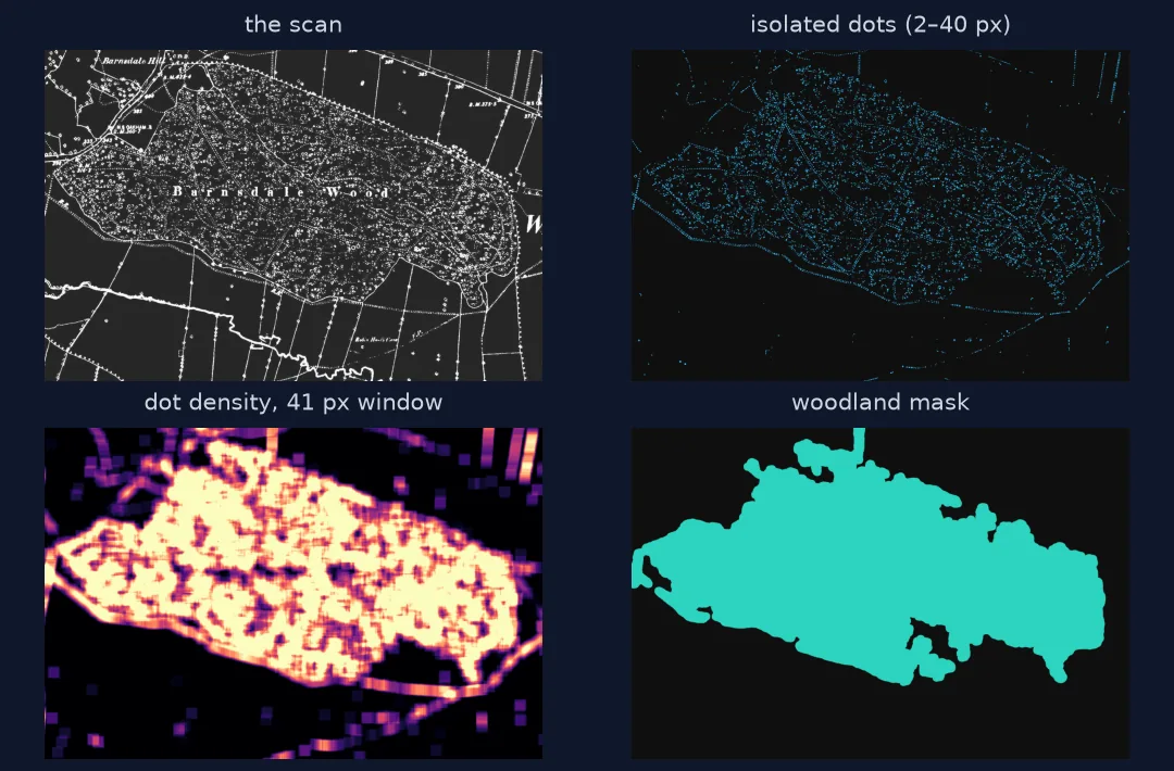
Every connected blob of ink on the scan has a size. Lines — roads, hedges, field boundaries, lettering — form large connected blobs; the tree symbols of a wood are dots of a few to a few dozen pixels:
print(f"{len(sizes) - 1:,} ink blobs; {is_dot.sum():,} of them 2-40 px; "
      f"dot pixels are {is_dot[lab].mean():.2%} of the sheet, all ink {(im < 128).mean():.1%}")
33,439 ink blobs; 24,789 of them 2-40 px; dot pixels are 1.35% of the sheet, all ink 8.1%
Dotted footpaths and the dots along hedgerows are also small blobs, so dots alone do not make a wood. Density does.
2. Turn dots into a density surface
A moving window counts the share of dot pixels around every pixel. Inside a wood the dots are everywhere; along a dotted path they are a thin line that a 41-pixel window (about 37 m) dilutes:
for label, (r, c) in {"inside Barnsdale Wood": (900, 3300), "open field": (2600, 600),
                      "Upper Hambleton village": (2050, 2200)}.items():
    print(f"{label:24} density {density[r, c]:.3f}")
inside Barnsdale Wood density 0.102
open field density 0.002
Upper Hambleton village density 0.008
A threshold of 0.04 sits between the two. Step 5 tests how much the answer depends on it.
3. Clean the mask by shape
An opening with a disc of radius 15 pixels removes anything narrower than about 27 m; filling holes closes the clearings and rides inside woods; and keeping only regions whose widest point is at least 35 pixels from an edge — about 60 m across — drops the last dotted lanes:
before = ndi.label(ndi.binary_fill_holes(ndi.binary_opening(density > 0.04, structure=DISK15)))[1]
print(f"{before} regions after the opening, {thick.sum()} thick enough to be woods")
217 regions after the opening, 15 thick enough to be woods
4. Vectorise and georeference
rasterio.features.shapes turns the mask into polygons in pixel coordinates; an affine transformation fitted to the sheet's corners — placed from the sheet layout — moves them to British National Grid:
print(woods.crs.to_epsg(), [round(v) for v in woods.total_bounds])
woods.to_file("data/woods_1880s.gpkg")
27700 [488620, 306383, 492855, 309387]
The polygons carry the georeferencing error of the sheet — about 20 m, measured at three churches — on top of the extraction's own.
5. Test the choices
Every number above was a choice. Changing each by a reasonable amount shows which ones matter:
def total_ha(threshold=0.04, window=41, radius=15):
    d = ndi.uniform_filter(is_dot[lab].astype(float), size=window)
    yy, xx = np.ogrid[-radius:radius + 1, -radius:radius + 1]
    m = ndi.binary_fill_holes(ndi.binary_opening(d > threshold, structure=xx**2 + yy**2 <= radius**2))
    Lm, km = ndi.label(m)
    m = np.r_[False, ndi.maximum(ndi.distance_transform_edt(m), Lm, range(1, km + 1)) >= 35][Lm]
    return to_polygons(m, "009-NE").area.sum() / 1e4

for kw in ({}, {"threshold": 0.03}, {"threshold": 0.05}, {"window": 31}, {"window": 61}, {"radius": 10}, {"radius": 20}):
    print(f"{str(kw or 'as chosen'):22} {total_ha(**kw):6.1f} ha")
as chosen 124.7 ha
{'threshold': 0.03} 153.3 ha
{'threshold': 0.05} 89.9 ha
{'window': 31} 105.6 ha
{'window': 61} 145.8 ha
{'radius': 10} 134.5 ha
{'radius': 20} 113.6 ha
The threshold matters most: 0.03 to 0.05 takes the total from 153 ha down to 90. The window moves it between 106 and 146 ha, the opening radius between 114 and 135, because both decide how far the edge of a wood extends past its outermost trees. Quote woodland area from a digitised old map with that range — about 90 to 150 ha here — not as a single number.
Woodland from the tree symbols of two sheets
The data used on this page
Ordnance Survey six-inch sheets Rutland 009-NW and 009-NE (1884–1891) from Wikimedia Commons (public domain). 009-NE is georeferenced from 009-NW's seven control points and the sheet layout, as in the mosaic guide.
from pathlib import Path

import geopandas as gpd
import numpy as np
import requests
from PIL import Image
from rasterio import features
from scipy import ndimage as ndi
from shapely import affinity
from shapely.geometry import shape

Path("data").mkdir(exist_ok=True)
UA = {"User-Agent": "spatialworkflow.io guide (https://www.spatialworkflow.io)"}
COMMONS = "https://upload.wikimedia.org/wikipedia/commons/"
for name, path in {"009-NW": "a/a0/", "009-NE": "8/80/"}.items():
    if not Path(f"data/os_{name}.jpg").exists():
        url = f"{COMMONS}{path}Map_of_Rutland_OS_Map_name_{name}%2C_Ordnance_Survey%2C_1884-1891.jpg"
        Path(f"data/os_{name}.jpg").write_bytes(requests.get(url, headers=UA, timeout=300).content)

GCPS = [  # (id, pixel, line, easting, northing) on 009-NW
    ("oakham_church",          3141,  487, 486065.6, 308906.1),
    ("egleton_church",         4824, 2031, 487598.5, 307540.3),
    ("brooke_rd_crossing",     2956, 1159, 485892.0, 308306.8),
    ("egleton_level_crossing", 3998, 2481, 486838.1, 307119.0),
    ("stamford_rd_guide_post", 5127,  988, 487872.3, 308486.1),
    ("braunston_rd_bridleway", 1263, 1675, 484382.4, 307839.2),
    ("brooke_guide_post",      1547, 3292, 484648.2, 306376.1),
]
SHEET_OFFSET = {"009-NW": 0, "009-NE": 1}
yy, xx = np.ogrid[-15:16, -15:16]
DISK15 = xx**2 + yy**2 <= 15**2

def sheet_affine(name):
    """Pixel -> British National Grid for a sheet, from 009-NW's fit and its place in the layout."""
    X = np.array([[1, g[1], g[2]] for g in GCPS], float)
    A = np.linalg.lstsq(X, np.array([[g[3], g[4]] for g in GCPS]), rcond=None)[0]
    w0, h0 = Image.open("data/os_009-NW.jpg").size
    w, h = Image.open(f"data/os_{name}.jpg").size
    sx, sy, off = w0 / w, h0 / h, SHEET_OFFSET[name] * w0
    # e = A0 + A1 * (off + c * sx) + A2 * (r * sy), likewise n
    return [A[1, 0] * sx, A[2, 0] * sy, A[1, 1] * sx, A[2, 1] * sy,
            A[0, 0] + A[1, 0] * off, A[0, 1] + A[1, 1] * off]

def to_polygons(mask, name):
    polys = [affinity.affine_transform(shape(p), sheet_affine(name))
             for p, _ in features.shapes(mask.astype(np.uint8), mask=mask)]
    g = gpd.GeoDataFrame(geometry=polys, crs=27700)
    return g[g.area > 2e4].reset_index(drop=True)                  # 2 ha and up

print({p.name: p.stat().st_size for p in Path("data").glob("os_*.jpg")})
{'os_009-NE.jpg': 3057362, 'os_009-NW.jpg': 2653911}
Example 1: what thresholding the ink alone gives you
For comparison, the naive approach: dark pixels, opened to remove thin lines, kept if large:
naive = ndi.binary_opening(im < 128, structure=np.ones((5, 5)))
nl, nk = ndi.label(naive)
big = np.r_[False, ndi.sum(naive, nl, range(1, nk + 1)) > 2000][nl]
print(f"{nk:,} solid blobs after opening; {ndi.label(big)[1]} over 2,000 px; "
      f"overlap with the woodland mask: {(big & mask).sum() / max(big.sum(), 1):.0%} of their pixels")
4,902 solid blobs after opening; 23 over 2,000 px; overlap with the woodland mask: 0% of their pixels
Solid ink is buildings, heavy lettering and the black of a railway cutting — almost none of it is woodland, because woods on these sheets are drawn light, not dark.
Example 2: export for QGIS and check by eye
Automated digitising should end with a look. A GeoPackage opens in QGIS over the warped sheet, where every edge can be checked against the scan:
woods["ha"] = (woods.area / 1e4).round(2)
woods["source"] = "OS six-inch Rutland 009-NE, 1884-1891, stipple density > 0.04"
woods.to_file("data/woods_1880s.gpkg", layer="woods")
print(gpd.read_file("data/woods_1880s.gpkg", layer="woods")[["ha", "source"]].head(3).to_string())
ha source
0 2.72 OS six-inch Rutland 009-NE, 1884-1891, stipple density > 0.04
1 9.10 OS six-inch Rutland 009-NE, 1884-1891, stipple density > 0.04
2 69.80 OS six-inch Rutland 009-NE, 1884-1891, stipple density > 0.04
Recording the method in the attribute table is what makes the polygons reusable: anyone opening the file later knows they were extracted, not traced, and from which sheet.
Map symbols are a code
Map symbols are a code, and digitising is decoding it. On a coloured modern map the code is mostly colour; on the black-and-white Ordnance Survey sheets of the 1880s it is shape, size and pattern. Buildings are solid, roads are pairs of lines, field boundaries single lines, hedgerow trees small circles at intervals, and woods a field of tree symbols. Thresholding reads only "is it ink", which is the one thing all of those share.
Texture measures work because they read the pattern instead. The connected-component sizes separate marks from lines; the window turns isolated marks into a property of an area; the opening and the thickness test encode what a wood is on the ground — wider than a lane, wider than a hedge. Each step encodes an assumption about the cartography, and each assumption is a number that step 5 can vary.
The result is not a tracing. Its edges follow the outermost tree symbols, smoothed by the window, rather than the boundary line the surveyor drew; small woods below the thickness threshold are missed; and a field of dots that is not a wood — a dense orchard, a parkland of scattered trees — would be found as one. That is why the method should be quoted with its range and checked by eye, and why, for a small area, tracing by hand is still the better tool.
Legends, scan resolution and lettering
- Read the legend first. The symbol code differs between series and editions; woods on later sheets carry tree symbols of different sizes.
- Scan resolution sets the pixel sizes. The 2–40 px dot range and 41 px window suit these scans at about 0.9 m per pixel; scale them for others.
- Parkland and orchards have tree symbols too; expect them to appear as woods.
- Lettering inside woods ("Barnsdale Wood") is a large blob, not a dot; filling holes covers it.
- Georeferencing error adds to extraction error. About 20 m here, before any edge effect.
- Record the method with the polygons.
Internal links
- How to measure change from an old map — these woods against Rutland Water
- How to mosaic historical map sheets — how 009-NE was placed
- Georeferencing explained — a georeferenced map is still a picture
- How accurate is a historical map? — the error the polygons inherit
- How to georeference a scanned map with GDAL — warping the sheet itself
FAQ
How do I extract features from a scanned map automatically?
Find what is distinctive about the symbol — here, woodland stipple made of many small isolated dots — measure it with connected-component sizes and a moving window, threshold, clean by shape, and vectorise with rasterio.features.shapes.
Why does thresholding a scanned map not work?
On a black-and-white map every feature is ink. Thresholding separates ink from paper, not woods from roads or buildings from lettering.
How accurate is automatically digitised woodland?
It depends on the choices; on sheet 009-NE, reasonable changes to the threshold, window and opening moved the total between 90 and 153 ha around a central 125 ha. Quote the range and check the outlines by eye.
Should I digitise old maps by hand instead?
For a few features, yes — a careful tracing follows the surveyor's boundary line. For a whole sheet or a series, a texture method with a stated range is faster and repeatable.