
Georeferencing Explained: Turning a Scanned Map into Spatial Data
On this page
Problem statement
A scanned map is a picture. Its pixels have a column and a row, and nothing else: the software that opens it has no idea that the black block at column 3141, row 487 is a church in Oakham, or that north on the paper is not quite north on the ground. Georeferencing is the step that gives every pixel a place, so the old map can sit on top of modern data, be measured, and be compared with the present.
This page explains what that step actually does, using the Ordnance Survey six-inch sheet of Oakham (surveyed 1884–1891) and seven control points matched to OpenStreetMap — the same sheet the rest of the historical maps guides use.
Quick answer
Georeferencing finds a function from pixel coordinates to map coordinates, fitted to a handful of points whose position you know in both, and then usually resamples the image onto a grid in the map's coordinate system:
t = gdal.Transformer(gdal.Open("data/os_gcps.vrt"), None, ["METHOD=GCP_POLYNOMIAL", "MAX_GCP_ORDER=1"])
ok, (e, n, _) = t.TransformPoint(0, 3141, 487)              # pixel -> British National Grid
lon, lat = Transformer.from_crs(27700, 4326, always_xy=True).transform(e, n)
print(f"pixel (3141, 487) -> E {e:,.1f}  N {n:,.1f} -> {lat:.5f} N, {abs(lon):.5f} W")
pixel (3141, 487) -> E 486,066.5 N 308,914.9 -> 52.67112 N, 0.72863 W
Three things went into that answer: the scan, the control points, and a choice of transformation. Each is a source of error, and the georeferenced map is only as good as the worst of them.
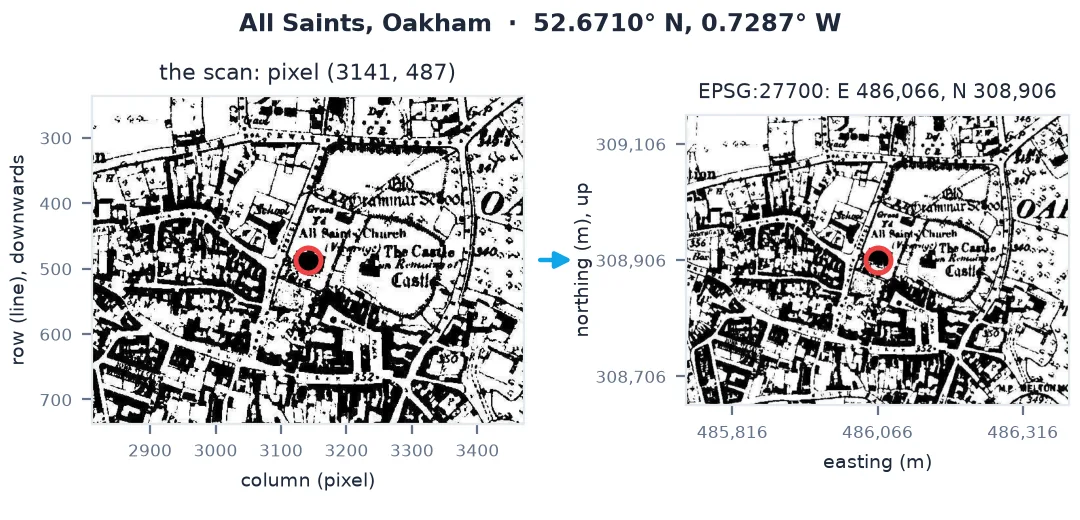
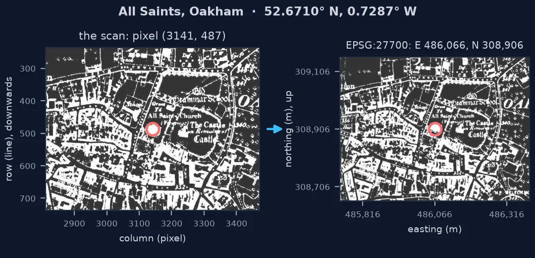
Pixel coordinates, control points, a transformation, a warp
1. Pixels have their own coordinate system
A raster's native coordinates count columns to the right and rows downwards from the top-left corner. Map coordinates count eastings to the right and northings upwards. Before georeferencing, the only "coordinates" a scan has are the first kind:
scan = gdal.Open("data/os_009-NW.jpg")
print("size:", scan.RasterXSize, "x", scan.RasterYSize, "| projection:", repr(scan.GetProjection()),
      "| geotransform:", scan.GetGeoTransform())
size: 5343 x 3573 | projection: '' | geotransform: (0.0, 1.0, 0.0, 0.0, 0.0, 1.0)
The identity geotransform — origin 0, one unit per pixel, y increasing downwards — is GDAL's way of saying "this is only an image".
2. Control points connect the two
A ground control point is a pair: a pixel on the scan and a coordinate on the ground, asserted to be the same place. Seven were picked on this sheet — churches, a guide post and railway crossings that exist both on the 1880s survey and in OpenStreetMap today:
for name, px, py, e, n in GCPS:
    print(f"{name:24} pixel ({px:4}, {py:4})  ->  E {e:9,.1f}  N {n:9,.1f}")
oakham_church pixel (3141, 487) -> E 486,065.6 N 308,906.1
egleton_church pixel (4824, 2031) -> E 487,598.5 N 307,540.3
brooke_rd_crossing pixel (2956, 1159) -> E 485,892.0 N 308,306.8
egleton_level_crossing pixel (3998, 2481) -> E 486,838.1 N 307,119.0
stamford_rd_guide_post pixel (5127, 988) -> E 487,872.3 N 308,486.1
braunston_rd_bridleway pixel (1263, 1675) -> E 484,382.4 N 307,839.2
brooke_guide_post pixel (1547, 3292) -> E 484,648.2 N 306,376.1
Everything that follows depends on these seven assertions being right. Ground control points explained covers what makes one trustworthy.
3. A transformation turns pixels into coordinates
With the points in place, a function is fitted to them. The simplest, an affine transformation, can only shift, scale, rotate and shear the sheet — and that is enough to read the map's geometry off its six coefficients:
P = np.array([[g[1], g[2], 1] for g in GCPS], float)
cx, *_ = np.linalg.lstsq(P, [g[3] for g in GCPS], rcond=None)
cy, *_ = np.linalg.lstsq(P, [g[4] for g in GCPS], rcond=None)
sx, sy = np.hypot(cx[0], cy[0]), np.hypot(cx[1], cy[1])
rot = np.degrees(np.arctan2(cy[0], cx[0]))
print(f"one pixel = {sx:.3f} m across, {sy:.3f} m down; rotated {rot:.2f} degrees from grid north")
print(f"sheet footprint: {sx * scan.RasterXSize / 1000:.2f} km x {sy * scan.RasterYSize / 1000:.2f} km")
one pixel = 0.903 m across, 0.900 m down; rotated 0.48 degrees from grid north
sheet footprint: 4.82 km x 3.22 km
About 0.9 m of ground per pixel, and a sheet turned by half a degree. The six-inch map's own sheet lines followed the Rutland county meridian, not the National Grid, which did not exist until the 1930s — so the rotation is real, not a scanning error.
4. The warp makes a new image in map coordinates
A function from pixels to coordinates is enough to look up a point. To use the map with other data it is usually resampled onto a north-up grid in the target coordinate system — the warp:
out = gdal.Warp("", "data/os_gcps.vrt", format="MEM", dstSRS="EPSG:27700", polynomialOrder=1,
                xRes=1, yRes=1, resampleAlg="cubic", dstAlpha=True)
gt = out.GetGeoTransform()
print("warped:", out.RasterXSize, "x", out.RasterYSize, "at", gt[1], "m | origin", round(gt[0]), round(gt[3]),
      "|", out.GetSpatialRef().GetName())
warped: 4843 x 3258 at 1.0 m | origin 483228 309370 | OSGB36 / British National Grid
5. Check the result against something you trust
A georeferenced map always lands somewhere. Whether it landed in the right place is a separate question, answered by predicting each control point from the others:
loo = []
for i, (name, px, py, e, n) in enumerate(GCPS):
    rest = GCPS[:i] + GCPS[i + 1:]
    A = np.array([[g[1], g[2], 1] for g in rest], float)
    fx, *_ = np.linalg.lstsq(A, [g[3] for g in rest], rcond=None)
    fy, *_ = np.linalg.lstsq(A, [g[4] for g in rest], rcond=None)
    loo.append(float(np.hypot(fx @ (px, py, 1) - e, fy @ (px, py, 1) - n)))
print("leave-one-out error:", [round(v, 1) for v in loo], "m; RMS", round(float(np.sqrt(np.mean(np.square(loo)))), 1), "m")
leave-one-out error: [16.5, 8.5, 14.6, 22.2, 21.8, 18.4, 16.9] m; RMS 17.5 m
Tens of metres, on a sheet surveyed at 1:10,560 well over a century ago. That number — not a residual, and not the pixel size — is the accuracy of the georeferenced map.
From modern features back to the old sheet
The data used on this page
The Ordnance Survey six-inch sheet Rutland 009-NW (1884–1891) from Wikimedia Commons (public domain), and seven control points matched to OpenStreetMap (Geofabrik, 1 January 2026; © OpenStreetMap contributors, ODbL).
from pathlib import Path

import geopandas as gpd
import numpy as np
import requests
from osgeo import gdal
from pyproj import Transformer

gdal.UseExceptions()
Path("data").mkdir(exist_ok=True)
UA = {"User-Agent": "spatialworkflow.io guide (https://www.spatialworkflow.io)"}
downloads = {
    "data/os_009-NW.jpg": "https://upload.wikimedia.org/wikipedia/commons/a/a0/"
                          "Map_of_Rutland_OS_Map_name_009-NW%2C_Ordnance_Survey%2C_1884-1891.jpg",
    "data/rutland.shp.zip": "https://download.geofabrik.de/europe/united-kingdom/england/rutland-260101-free.shp.zip",
}
for target, url in downloads.items():
    if not Path(target).exists():
        Path(target).write_bytes(requests.get(url, headers=UA, timeout=300).content)
jpg = Path("data/os_009-NW.jpg")
GCPS = [  # (id, pixel, line, easting, northing)
    ("oakham_church",          3141,  487, 486065.6, 308906.1),
    ("egleton_church",         4824, 2031, 487598.5, 307540.3),
    ("brooke_rd_crossing",     2956, 1159, 485892.0, 308306.8),
    ("egleton_level_crossing", 3998, 2481, 486838.1, 307119.0),
    ("stamford_rd_guide_post", 5127,  988, 487872.3, 308486.1),
    ("braunston_rd_bridleway", 1263, 1675, 484382.4, 307839.2),
    ("brooke_guide_post",      1547, 3292, 484648.2, 306376.1),
]
gdal.Translate("data/os_gcps.vrt", str(jpg), format="VRT", bandList=[1], outputSRS="EPSG:27700",
               GCPs=[gdal.GCP(e, n, 0, px, py, name) for name, px, py, e, n in GCPS])
print(jpg.stat().st_size, "bytes;", len(GCPS), "control points")
2653911 bytes; 7 control points
Example 1: going the other way — where is a modern feature on the old map?
The same transformation runs backwards. Oakham railway station's position today, looked up on the 1880s scan:
osm = gpd.read_file("/vsizip/data/rutland.shp.zip/gis_osm_transport_free_1.shp",
                    bbox=(-0.75, 52.66, -0.72, 52.68)).to_crs(27700)
station = osm[osm["fclass"] == "railway_station"].iloc[0]
ok, (col, row, _) = t.TransformPoint(1, station.geometry.x, station.geometry.y)   # 1 = inverse
print(station["name"], "->", f"column {col:.0f}, row {row:.0f}")
Oakham -> column 2712, row 346
The answer lands on the railway beside the word "Station" on the 1880s sheet — the station has not moved since 1848. This is how a georeferenced map is used without being warped: look up modern features on the original scan, at its full resolution, with no resampling at all.
Example 2: a georeferenced map is still a picture
Georeferencing places the pixels; it does not tell the computer what they show. Reading the warped sheet's values at the church and in an open field gives brightness — 0 for ink, 255 for paper — not "church" and "field":
warped = gdal.Warp("", "data/os_gcps.vrt", format="MEM", dstSRS="EPSG:27700", polynomialOrder=1, xRes=1, yRes=1)
gt = warped.GetGeoTransform()
band = warped.GetRasterBand(1).ReadAsArray()
for label, (e, n) in {"All Saints church": (486065.6, 308906.1), "a field south-west of the town": (485500, 307400)}.items():
    c, r = int((e - gt[0]) / gt[1]), int((n - gt[3]) / gt[5])
    print(f"{label:28} grey value {band[r, c]}")
All Saints church grey value 0
a field south-west of the town grey value 255
Turning ink into features — roads, buildings, field boundaries with attributes — is a separate step, digitising.
What every georeferencing workflow shares
Every georeferencing workflow, in QGIS, ArcGIS, GDAL or a web tool, has the same structure: control points in, a fitted transformation, an optional resampling onto a new grid. The tools differ in how you click; the mathematics underneath is the same, and so are the ways it goes wrong.
It helps to separate three kinds of error, because they need different fixes:
- Errors in the map. A Victorian surveyor working with chains and theodolites placed features to within metres, and the paper has since stretched and shrunk with damp. No transformation can remove what is in the original; it can only spread it evenly.
- Errors in the matching. A control point says "this pixel is that place". If the place has moved — a church rebuilt, a road widened — or the pixel was clicked carelessly, the transformation fits a falsehood.
- Errors in the model. An affine transformation cannot bend; a polynomial can bend too much; a spline will bend exactly as far as your mistakes ask it to.
Georeferencing also has a direction worth keeping in mind. Fitting goes from points to a function; warping uses the function backwards, asking for every cell of the new grid where it came from on the scan. That is why warped maps have empty corners, why the resampling method matters, and why the output's resolution is a choice rather than a property of the scan.
Finally, a georeferenced historical map carries two dates: the date of the survey and the date of the data you matched it to. Any measurement of change — a field boundary that moved, a river that shifted — has to be larger than the tens of metres of georeferencing error to mean anything.
Downward rows, small rotations and projections
- Pixel rows run downwards, map northings upwards; a sign error flips the map.
- A rotation of a few tenths of a degree is normal for maps drawn on a pre-national-grid sheet layout.
- Georeferencing does not change the map's projection; it fits whatever projection the map was drawn in to yours. For maps drawn on unusual projections see old map projections explained.
- Residuals are not accuracy. Leave-one-out error or independent check points are.
- A georeferenced map is still a picture; to analyse its features, digitise them.
Internal links
- Ground control points explained — what makes a point trustworthy
- Georeferencing transformations explained — affine, polynomial and spline in detail
- How to georeference a scanned map with GDAL in Python — the practical recipe
- How accurate is a historical map? — the limits that come from the original survey
- How to download scanned historical maps — where the Oakham sheet came from
FAQ
What does georeferencing mean?
Assigning real-world coordinates to an image, by fitting a function from its pixels to a coordinate system using control points — positions you can identify on both the image and the ground.
Is georeferencing the same as rectification?
Nearly. Georeferencing is finding the function; rectification (or warping) is using it to resample the image onto a new grid in the target coordinate system. Most tools do both in one step.
How many control points do I need?
Three is the mathematical minimum for an affine fit. In practice six to ten well-spread points let you test each one against the rest; this page uses seven on a sheet 5 km wide.
How accurate is a georeferenced old map?
Measure it rather than assume it. On the Oakham sheet, predicting each control point from the others gives errors of 8 to 22 m.
Can I georeference without warping?
Yes. Keep the control points in the file (a VRT or GCPs in a GeoTIFF) or store an affine geotransform, and look up coordinates as needed. Warp when you need a north-up grid for other software.