Georeferencing Transformations Explained: Affine, Polynomial and Thin-Plate Spline

Problem statement

A transformation is the formula that turns a scan's column and row into a map coordinate. An affine one has six coefficients and can only shift, rotate, scale and shear the sheet, so straight lines stay straight and parallel ones stay parallel; a second-order polynomial has twelve and can curve them; a thin-plate spline adds one weight per control point to an affine part, passes through every point exactly and bends the sheet freely in between. The number of coefficients, set against the number of control points, decides what a transformation can fit and what it can invent.

This page writes out the three transformations GDAL and QGIS use most, fits each by hand in NumPy to the seven control points on the Ordnance Survey six-inch sheet of Oakham (1884–1891), checks the hand-made versions against GDAL, and shows what each one does to the corners of the sheet.

Quick answer

An affine transformation is two linear equations with six coefficients; a second-order polynomial adds squared and cross terms for twelve; a thin-plate spline adds one weight per control point on top of an affine part:

P = np.array([[px, py] for _, px, py, _, _ in GCPS], float)
W = np.array([[e, n] for *_, e, n in GCPS], float)

for label, X in {"affine": design(P, 1), "polynomial 2": design(P, 2)}.items():
    coef, *_ = np.linalg.lstsq(X, W, rcond=None)
    resid = np.hypot(*(X @ coef - W).T)
    print(f"{label:13} {coef.size:2} coefficients from {len(P)} points; residual RMS {np.sqrt(np.mean(resid**2)):5.2f} m")
tps = fit_tps(P, W)
print(f"{'spline':13} {tps['w'].size + tps['a'].size:2} coefficients from {len(P)} points; residual RMS "
      f"{np.sqrt(np.mean(np.hypot(*(apply_tps(tps, P) - W).T) ** 2)):5.2f} m")

affine         6 coefficients from 7 points; residual RMS 10.18 m
polynomial 2  12 coefficients from 7 points; residual RMS  1.87 m
spline        20 coefficients from 7 points; residual RMS  0.00 m

More coefficients, smaller residuals — and less reason to trust them, because a transformation with as many coefficients as constraints can fit anything. What the extra freedom does is clearest at the edges of the sheet, where there are no points to hold it:

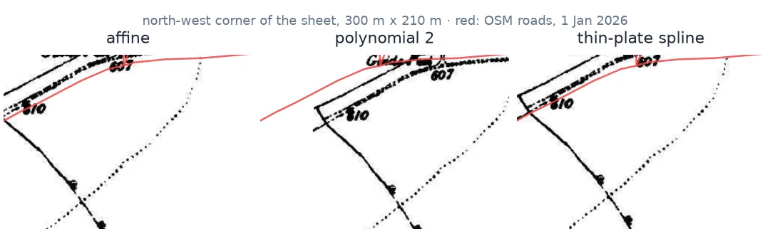
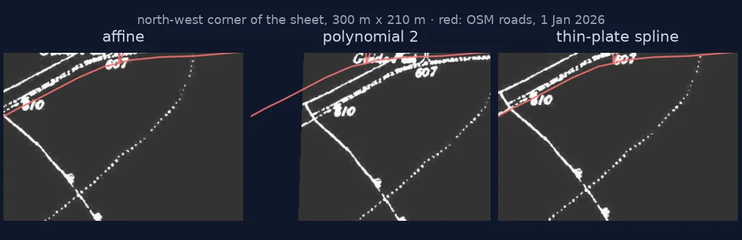
Affine planes, polynomial curvature, exact splines

1. Affine: a tilted plane for each coordinate

An affine transformation computes easting and northing each as a weighted sum of column, row and a constant. Its six coefficients decompose into things you can name — scale, rotation, shear and shift:

A, *_ = np.linalg.lstsq(design(P, 1), W, rcond=None)      # rows: 1, column, row
(e0, n0), (a, d), (b, c) = A
sx, sy = np.hypot(a, d), np.hypot(b, c)
rotation = np.degrees(np.arctan2(d, a))
shear = np.degrees(np.arccos(abs(a * b + d * c) / (sx * sy)))   # 90 means no shear
print(f"origin E {e0:,.0f} N {n0:,.0f}; scale {sx:.4f} x {sy:.4f} m/pixel; rotation {rotation:.2f} deg; axes meet at {shear:.2f} deg")

origin E 483,228 N 309,330; scale 0.9028 x 0.9004 m/pixel; rotation 0.48 deg; axes meet at 89.86 deg

Straight lines stay straight and parallels stay parallel. Shear lets the two axes meet at something other than a right angle; here they meet at almost exactly 90°, so the scan is square and the only real distortions are scale and the half-degree turn of the old sheet layout against the National Grid. A Helmert (similarity) transformation is affine without shear and with one scale; a projective one lets parallels converge, which suits a photograph of a map taken at an angle.

2. Polynomial: curvature from extra terms

A second-order polynomial adds column², row² and column×row to each equation. The extra terms let the sheet bow — and with only seven points, the curvature is decided by very little evidence:

X2 = design(P, 2)
print("condition number, affine:", f"{np.linalg.cond(design(P, 1)):,.0f}", "| polynomial 2:", f"{np.linalg.cond(X2):,.0f}")
coef2, *_ = np.linalg.lstsq(X2, W, rcond=None)
corner = design(np.array([[0.0, 0.0], [5343.0, 3573.0]]), 2) @ coef2 - design(np.array([[0.0, 0.0], [5343.0, 3573.0]]), 1) @ A
print("polynomial minus affine at the top-left and bottom-right corners:", np.round(np.hypot(*corner.T), 1), "m")

condition number, affine: 14,675 | polynomial 2: 457,698,259
polynomial minus affine at the top-left and bottom-right corners: [90.  49.4] m

A condition number in the hundreds of millions means small changes in the points cause large changes in the coefficients. Inside the cloud of points the polynomial and the affine fit agree to within metres; at the corners, where nothing constrains the squared terms, they part by tens of metres.

3. Thin-plate spline: exact at the points, smooth between

A thin-plate spline is the affine fit plus a sum of radial functions, one centred on each control point, with weights chosen so it passes exactly through every point while bending as little as possible. The whole thing is one linear system — fit_tps and apply_tps in the setup block below are a complete implementation in fifteen lines. Checked against GDAL's own spline:

tps = fit_tps(P, W)
gdal_tps = gdal.Transformer(gdal.Open("data/os_gcps.vrt"), None, ["METHOD=GCP_TPS"])
probe = np.array([[100.0, 100.0], [2600.0, 1800.0], [5200.0, 3400.0]])
ours = apply_tps(tps, probe)
theirs = np.array([gdal_tps.TransformPoint(0, *p)[1][:2] for p in probe])
print("ours - GDAL at three pixels:", np.round(np.hypot(*(ours - theirs).T), 3), "m")

ours - GDAL at three pixels: [0. 0. 0.] m

The hand-written spline matches GDAL's to under a millimetre. Between and beyond the points it stays close to the least-squares affine fit — within 20 m everywhere on this sheet, as Example 2 measures — which is why it cannot run away at the edges the way a polynomial can.

4. Compare by prediction, not by residual

Residuals favour freedom. Predicting each point from the other six favours whatever actually describes the map:

def loo(fit_predict):
    return [float(np.hypot(*(fit_predict(np.delete(P, i, 0), np.delete(W, i, 0), P[i:i + 1])[0] - W[i])))
            for i in range(len(P))]

methods = {
    "affine": lambda p, w, x: design(x, 1) @ np.linalg.lstsq(design(p, 1), w, rcond=None)[0],
    "polynomial 2": lambda p, w, x: design(x, 2) @ np.linalg.lstsq(design(p, 2), w, rcond=None)[0],
    "thin-plate spline": lambda p, w, x: apply_tps(fit_tps(p, w), x),
}
for label, f in methods.items():
    e = loo(f)
    print(f"{label:18} leave-one-out RMS {np.sqrt(np.mean(np.square(e))):7.1f} m  worst {max(e):7.1f} m")

affine             leave-one-out RMS    17.5 m  worst    22.2 m
polynomial 2       leave-one-out RMS   571.1 m  worst  1509.9 m
thin-plate spline  leave-one-out RMS    11.6 m  worst    16.7 m

The same ranking GDAL's own transformers gave in the comparison guide: the spline predicts best on this sheet, the affine fit close behind, and the polynomial — which needs six points and gets exactly six in each leave-one-out fit — fails badly.

Hand-made and GDAL affine fits compared

The data used on this page

The seven control points picked on the Ordnance Survey six-inch sheet Rutland 009-NW (1884–1891, Wikimedia Commons, public domain) against OpenStreetMap (Geofabrik, 1 January 2026; © OpenStreetMap contributors, ODbL), and the scan itself for the GDAL comparison.

from pathlib import Path

import numpy as np
import requests
from osgeo import gdal

gdal.UseExceptions()
Path("data").mkdir(exist_ok=True)
UA = {"User-Agent": "spatialworkflow.io guide (https://www.spatialworkflow.io)"}
jpg = Path("data/os_009-NW.jpg")
if not jpg.exists():
    jpg.write_bytes(requests.get("https://upload.wikimedia.org/wikipedia/commons/a/a0/"
                                 "Map_of_Rutland_OS_Map_name_009-NW%2C_Ordnance_Survey%2C_1884-1891.jpg",
                                 headers=UA, timeout=300).content)
GCPS = [  # (id, pixel, line, easting, northing)
    ("oakham_church",          3141,  487, 486065.6, 308906.1),
    ("egleton_church",         4824, 2031, 487598.5, 307540.3),
    ("brooke_rd_crossing",     2956, 1159, 485892.0, 308306.8),
    ("egleton_level_crossing", 3998, 2481, 486838.1, 307119.0),
    ("stamford_rd_guide_post", 5127,  988, 487872.3, 308486.1),
    ("braunston_rd_bridleway", 1263, 1675, 484382.4, 307839.2),
    ("brooke_guide_post",      1547, 3292, 484648.2, 306376.1),
]
gdal.Translate("data/os_gcps.vrt", str(jpg), format="VRT", bandList=[1], outputSRS="EPSG:27700",
               GCPs=[gdal.GCP(e, n, 0, px, py) for _, px, py, e, n in GCPS])

def design(P, order):
    """Polynomial design matrix in column and row: order 1 -> 1, x, y; order 2 adds x^2, xy, y^2."""
    x, y = P[:, 0], P[:, 1]
    cols = [np.ones(len(P)), x, y]
    if order >= 2:
        cols += [x * x, x * y, y * y]
    return np.column_stack(cols)

def fit_tps(P, W):
    """Thin-plate spline P -> W: U(r) = r^2 log r kernels plus an affine part."""
    n = len(P)
    r = np.hypot(*(P[:, None, :] - P[None, :, :]).transpose(2, 0, 1))
    K = np.where(r > 0, r**2 * np.log(np.where(r > 0, r, 1)), 0)
    Q = np.c_[np.ones(n), P]
    L = np.block([[K, Q], [Q.T, np.zeros((3, 3))]])
    sol = np.linalg.solve(L, np.r_[W, np.zeros((3, 2))])
    return {"P": P, "w": sol[:n], "a": sol[n:]}

def apply_tps(t, X):
    r = np.hypot(*(X[:, None, :] - t["P"][None, :, :]).transpose(2, 0, 1))
    U = np.where(r > 0, r**2 * np.log(np.where(r > 0, r, 1)), 0)
    return U @ t["w"] + np.c_[np.ones(len(X)), X] @ t["a"]

print(len(GCPS), "control points")

7 control points

Example 1: the hand-made affine fit is GDAL's affine fit

GDAL's GCP_POLYNOMIAL with order 1 is the same least-squares fit:

gdal_aff = gdal.Transformer(gdal.Open("data/os_gcps.vrt"), None, ["METHOD=GCP_POLYNOMIAL", "MAX_GCP_ORDER=1"])
ours = design(probe, 1) @ A
theirs = np.array([gdal_aff.TransformPoint(0, *p)[1][:2] for p in probe])
print("ours - GDAL:", np.round(np.hypot(*(ours - theirs).T), 4), "m")

ours - GDAL: [0. 0. 0.] m

Knowing the transformation is a short piece of linear algebra makes it easy to reproduce, test and explain — and to see that nothing about it is specific to maps.

Example 2: where the spline bends

The spline's departure from the least-squares affine fit shows where it is bending the sheet to honour the points:

gx, gy = np.meshgrid(np.linspace(0, 5343, 54), np.linspace(0, 3573, 36))
G = np.c_[gx.ravel(), gy.ravel()]
bend = np.hypot(*(apply_tps(tps, G) - design(G, 1) @ A).T)
print(f"spline minus affine fit: median {np.median(bend):.1f} m, max {bend.max():.1f} m")
for name, px, py, *_ in GCPS:
    i = np.argmin(np.hypot(G[:, 0] - px, G[:, 1] - py))
    print(f"  near {name:24} {bend[i]:5.1f} m")

spline minus affine fit: median 9.7 m, max 19.6 m
  near oakham_church              8.7 m
  near egleton_church             5.3 m
  near brooke_rd_crossing        10.8 m
  near egleton_level_crossing    14.0 m
  near stamford_rd_guide_post    12.6 m
  near braunston_rd_bridleway     9.1 m
  near brooke_guide_post          5.9 m

The bending is 5 to 20 m, largest near the points the affine fit misses most — Egleton level crossing and the Stamford Road guide post — and the same size as the leave-one-out errors. The spline is using its freedom on real distortion in the map, which is why it predicts better here; given a misplaced point, it would use the same freedom to bend towards the mistake.

All three are fitted the same way

All three transformations are fitted the same way — by solving a linear system built from the control points — and differ only in which shapes they are allowed to produce:

• Affine maps rectangles to parallelograms. It captures everything a well-made map scan usually needs: the map's scale, its rotation against the grid, a small shear from paper and scanner. With more points than its three-point minimum it averages out the noise in them.
• Polynomial (order 2 or 3) allows smooth bowing across the sheet. That fits real distortion when it is systematic — a map drawn on a projection different from yours, or a sheet that shrank more along one axis — but its curvature is global: one point's error bends the whole sheet, and the bending grows fastest outside the points.
• Thin-plate spline allows local bending around each point, with the minimum total bending needed to hit every point exactly. Its freedom is spent near the points, not at the edges, and it has no residuals to check against — so it is only as good as the worst point.

The practical rule follows: start with affine; move to a spline when you have enough checked points that leave-one-out shows it predicts better; use a polynomial only when you have many points around the edges of the sheet and a reason to expect smooth distortion. On the Oakham sheet the spline wins, the affine fit is a close and safer second, and the polynomial is unusable with seven points.

QGIS's linear option, projective fits and conditioning

• QGIS's "Linear" is a scale-and-shift without rotation, not a full affine; "Helmert" adds rotation and one scale; "Polynomial 1" is the full affine.
• Projective handles perspective — a map photographed at an angle — not paper distortion.
• Polynomial order 3 needs 10 points and is rarely justified on a single sheet.
• The spline needs no minimum beyond three, but every point is honoured exactly, mistakes included.
• Condition numbers in the hundreds of millions mean the polynomial's coefficients are poorly determined; centring and scaling the pixel coordinates helps numerically but not statistically.
• Transformations are fitted pixel to world for warping; GDAL also fits or inverts the reverse for each output cell.

Internal links

• How to compare georeferencing transformations — the same three, scored with GDAL
• Georeferencing explained — the whole process
• Ground control points explained — the input every transformation depends on
• How to draw a distortion grid for an old map — seeing the bending as a deformed grid
• Warped map is folded or stretched — what too much freedom looks like

FAQ

What is the difference between affine and polynomial georeferencing?

Affine is polynomial order 1: six coefficients, straight lines stay straight. Order 2 adds three squared and cross terms per coordinate, allowing the sheet to bow, and needs at least six points.

What does a thin-plate spline transformation do?

It passes exactly through every control point and bends the image as little as possible in between, behaving like an affine fit far from the points.

Which georeferencing transformation is most accurate?

Whichever predicts held-out points best on your map. On the seven-point Oakham sheet: thin-plate spline 11.6 m RMS, affine 17.5 m, polynomial 2 over 500 m.

Why does my polynomial transformation distort the edges?

Its squared terms are constrained only where there are points. Outside the cloud of control points they extrapolate, and the distortion grows quickly towards the corners.