
How to Compare Georeferencing Transformations in Python
On this page
Problem statement
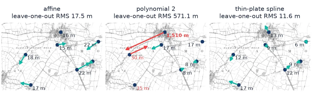
Seven control points on the Ordnance Survey six-inch sheet of Oakham (1884–1891) are enough to fit an affine transformation, a second-order polynomial and a thin-plate spline, and each reports a residual. The thin-plate spline reports zero, because it passes through every point; the polynomial reports almost zero while putting a church a kilometre and a half from where it stands. A residual measured on the points a transformation was fitted to cannot rank them — predicting each point from the other six can.
Quick answer
Fit each transformation with GDAL and score it by leave-one-out error, not by its residuals:
def fit(points, opts):
    """GDAL's pixel -> British National Grid transformer, fitted to `points`."""
    vrt = gdal.Translate("", "data/os_009-NW.jpg", format="VRT", bandList=[1], outputSRS="EPSG:27700",
                         GCPs=[gdal.GCP(e, n, 0, px, py) for _, px, py, e, n in points])
    t = gdal.Transformer(vrt, None, opts)
    t.vrt = vrt                                   # keep the dataset alive with the transformer
    return t

def errors(t, points):
    """Distance in metres between where `t` puts each point and where it was surveyed."""
    return [float(np.hypot(*(np.array(t.TransformPoint(0, px, py)[1][:2]) - (e, n)))) for _, px, py, e, n in points]

def rms(v):
    return float(np.sqrt(np.mean(np.square(v))))

METHODS = {"affine": ["METHOD=GCP_POLYNOMIAL", "MAX_GCP_ORDER=1"],
           "polynomial 2": ["METHOD=GCP_POLYNOMIAL", "MAX_GCP_ORDER=2"],
           "thin-plate spline": ["METHOD=GCP_TPS"]}

for label, opts in METHODS.items():
    resid = errors(fit(GCPS, opts), GCPS)
    loo = [errors(fit(GCPS[:i] + GCPS[i + 1:], opts), [g])[0] for i, g in enumerate(GCPS)]
    print(f"{label:18} residual RMS {rms(resid):6.1f} m   leave-one-out RMS {rms(loo):7.1f} m")
affine residual RMS 10.2 m leave-one-out RMS 17.5 m
polynomial 2 residual RMS 1.9 m leave-one-out RMS 571.1 m
thin-plate spline residual RMS 0.0 m leave-one-out RMS 11.6 m
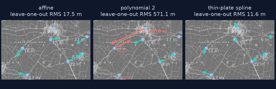
The residuals rank the three in the wrong order. Predicting each point from the other six ranks them in the right one — and shows that the polynomial, with seven points, is unusable:
One fit function, point minimums, leave-one-out errors
1. Wrap the fit in a function
The three functions in the quick answer do all the work. fit builds GDAL's Transformer, which uses exactly the code gdal.Warp uses, so a score computed with it applies to the warped file. errors measures distances in metres; here are the affine fit's residuals at the seven points:
print([round(v, 1) for v in errors(fit(GCPS, METHODS["affine"]), GCPS)])[8.8, 5.1, 11.2, 14.6, 12.5, 9.6, 5.7]
2. Know how many points each method needs
An affine transformation has 6 unknowns and needs 3 points; a second-order polynomial has 12 and needs 6; third order needs 10. Ask for more than the points allow and GDAL refuses:
for order in (1, 2, 3):
    try:
        fit(GCPS, ["METHOD=GCP_POLYNOMIAL", f"MAX_GCP_ORDER={order}"])
        print(order, "fitted")
    except RuntimeError as err:
        print(order, "refused:", str(err).splitlines()[0][:80])
1 fitted
2 fitted
3 refused: Failed to compute GCP transform: Not enough points available
Leaving one point out of seven leaves six — exactly the minimum for order 2. A polynomial fitted to exactly as many points as it has terms passes through every one of them and is free to do anything in between and beyond.
3. Compare leave-one-out errors point by point
table = pd.DataFrame({label: [errors(fit(GCPS[:i] + GCPS[i + 1:], opts), [g])[0] for i, g in enumerate(GCPS)]
                      for label, opts in METHODS.items()}, index=[g[0] for g in GCPS]).round(1)
print(table)
affine polynomial 2 thin-plate spline
oakham_church 16.5 1509.9 12.8
egleton_church 8.5 7.8 8.6
brooke_rd_crossing 14.6 17.0 8.7
egleton_level_crossing 22.2 8.0 12.1
stamford_rd_guide_post 21.8 17.4 6.3
braunston_rd_bridleway 18.4 29.7 12.5
brooke_guide_post 16.9 34.6 16.7
The polynomial does well where it is interpolating and catastrophically at Oakham church, the point nearest the top edge: leave it out and the remaining six say nothing about that corner, so the curve extrapolates freely. The thin-plate spline beats the affine fit at six of the seven points.
4. See where the methods disagree across the sheet
Leave-one-out tests only where you have points. To see the rest of the sheet, compare each method with the affine fit on a grid:
w, h = Image.open("data/os_009-NW.jpg").size
xs, ys = np.meshgrid(np.linspace(0, w, 108), np.linspace(0, h, 72))
grid = np.c_[xs.ravel(), ys.ravel(), np.zeros(xs.size)].tolist()
base = np.array(fit(GCPS, METHODS["affine"]).TransformPoints(0, grid)[0])[:, :2]
for label in ("polynomial 2", "thin-plate spline"):
    d = np.hypot(*(np.array(fit(GCPS, METHODS[label]).TransformPoints(0, grid)[0])[:, :2] - base).T)
    print(f"{label:18} median {np.median(d):5.1f} m  max {d.max():5.1f} m  over 20 m: {(d > 20).mean():.0%}")
polynomial 2 median 14.7 m max 90.0 m over 20 m: 28%
thin-plate spline median 9.6 m max 19.6 m over 20 m: 0%
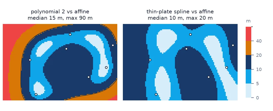
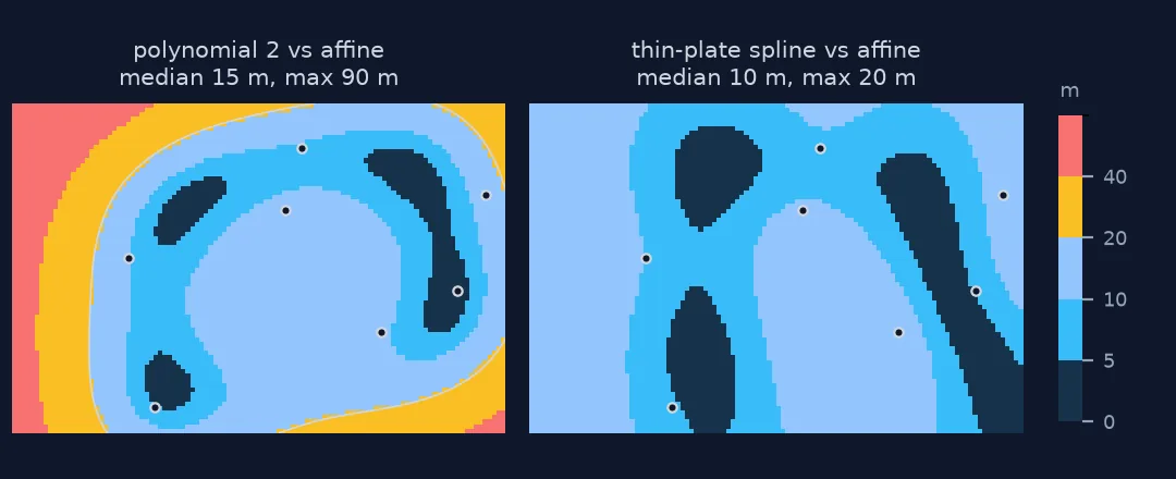
The spline bends the sheet by up to 20 m, and only where its control points ask it to. The polynomial bends hardest at the edges, where there are no points at all — 28% of the sheet sits more than 20 m from the affine result.
5. Choose, and warp
With seven points on one six-inch sheet, a thin-plate spline gives the lowest prediction error and the affine fit is the safe fallback; the second-order polynomial should not be used. Warp with the choice:
for label, kw in (("affine", dict(polynomialOrder=1)), ("tps", dict(tps=True))):
    t0 = time.perf_counter()
    gdal.Warp(f"data/oakham_{label}.tif", "data/os_gcps.vrt", dstSRS="EPSG:27700", xRes=1, yRes=1,
              resampleAlg="cubic", dstAlpha=True, creationOptions=["COMPRESS=DEFLATE", "TILED=YES", "PREDICTOR=2"], **kw)
    print(f"{label:7} {time.perf_counter() - t0:4.1f} s  {os.path.getsize(f'data/oakham_{label}.tif') / 1e6:.1f} MB")
affine 1.3 s 5.2 MB
tps 1.3 s 5.1 MB
Comparing transformations in pixels and with a bad point
The data used on this page
The Ordnance Survey six-inch sheet Rutland 009-NW (1884–1891) from Wikimedia Commons (public domain), and the seven control points picked against OpenStreetMap (Geofabrik, 1 January 2026; © OpenStreetMap contributors, ODbL) in the control-point guide.
import os
import time
from pathlib import Path

import numpy as np
import pandas as pd
import requests
from osgeo import gdal
from PIL import Image

gdal.UseExceptions()
Path("data").mkdir(exist_ok=True)
UA = {"User-Agent": "spatialworkflow.io guide (https://www.spatialworkflow.io)"}
scan = Path("data/os_009-NW.jpg")
if not scan.exists():
    scan.write_bytes(requests.get("https://upload.wikimedia.org/wikipedia/commons/a/a0/"
                                  "Map_of_Rutland_OS_Map_name_009-NW%2C_Ordnance_Survey%2C_1884-1891.jpg",
                                  headers=UA, timeout=300).content)
GCPS = [  # (id, pixel, line, easting, northing)
    ("oakham_church",          3141,  487, 486065.6, 308906.1),
    ("egleton_church",         4824, 2031, 487598.5, 307540.3),
    ("brooke_rd_crossing",     2956, 1159, 485892.0, 308306.8),
    ("egleton_level_crossing", 3998, 2481, 486838.1, 307119.0),
    ("stamford_rd_guide_post", 5127,  988, 487872.3, 308486.1),
    ("braunston_rd_bridleway", 1263, 1675, 484382.4, 307839.2),
    ("brooke_guide_post",      1547, 3292, 484648.2, 306376.1),
]
gdal.Translate("data/os_gcps.vrt", str(scan), format="VRT", bandList=[1], outputSRS="EPSG:27700",
               GCPs=[gdal.GCP(e, n, 0, px, py) for _, px, py, e, n in GCPS])
print(Image.open(scan).size, len(GCPS), "control points")
(5343, 3573) 7 control points
Example 1: the same comparison in pixels, as QGIS reports it
QGIS's georeferencer reports residuals in pixels of the scan. Converting is a matter of the scale — about 1.1 pixels per metre on this sheet — but the ranking is the point:
scale = np.hypot(*(np.array(GCPS[1][1:3]) - GCPS[0][1:3])) / np.hypot(*(np.array(GCPS[1][3:]) - GCPS[0][3:]))
for label, opts in METHODS.items():
    r = errors(fit(GCPS, opts), GCPS)
    print(f"{label:18} mean residual {np.mean(r) * scale:5.1f} px")
affine mean residual 10.7 px
polynomial 2 mean residual 1.7 px
thin-plate spline mean residual 0.0 px
A thin-plate spline's residuals are always zero by construction — it passes through every point. A table of residuals in which one method scores 0.0 is not evidence that the method is best; it is evidence that the table measures nothing for that method.
Example 2: what one bad point does to each method
Move one control point 60 pixels, as a slip of the mouse would, and see which method notices:
bad = list(GCPS)
name, px, py, e, n = bad[2]
bad[2] = (name, px + 60, py, e, n)
for label, opts in METHODS.items():
    loo = [errors(fit(bad[:i] + bad[i + 1:], opts), [g])[0] for i, g in enumerate(bad)]
    print(f"{label:18} residual RMS {rms(errors(fit(bad, opts), bad)):6.1f} m   worst leave-one-out {max(loo):7.1f} m at {bad[int(np.argmax(loo))][0]}")
affine residual RMS 24.5 m worst leave-one-out 68.6 m at brooke_rd_crossing
polynomial 2 residual RMS 4.2 m worst leave-one-out 1418.6 m at oakham_church
thin-plate spline residual RMS 0.0 m worst leave-one-out 64.2 m at oakham_church
The affine fit points straight at the culprit: its worst leave-one-out error is the moved point, 68.6 m against 14.6 m before. The thin-plate spline's residual stays at zero — it bends the map to honour the mistake. Its leave-one-out errors do jump, from a worst of 17 m to 64 m, so something is wrong; but the worst score lands on Oakham church, not on the point that moved. The polynomial's scores were already meaningless.
So find bad points with an affine fit, and only then fit a spline to the points that survive.
Every transformation is a function from scan to ground
Every georeferencing transformation is a function from scan pixels to map coordinates, fitted to the control points. They differ in how much freedom they have:
- Affine (polynomial order 1) can shift, scale, rotate and shear the sheet, but straight lines stay straight and parallel lines stay parallel. It cannot follow paper that has stretched more in one corner than another, but it also cannot do anything wild.
- Polynomial order 2 adds curvature — 12 coefficients that let the sheet bow. With many well-spread points it can model a survey's systematic distortion; with few, it fits the points and invents the rest.
- Thin-plate spline passes exactly through every point and bends the sheet as little as possible in between. Its freedom is local: far from any point it falls back to an affine fit, which is why it cannot run away at the edges the way a polynomial does.
Residuals measure how closely a function passes through the points it was fitted to, which says more about the function's freedom than about the map. Leave-one-out measures how well it predicts a point it has not seen — the only kind of point the rest of the sheet consists of.
On the Oakham sheet the spline wins, because the Victorian survey and the paper both carry small local distortions that an affine fit cannot follow. On a sheet with poorly placed or poorly matched points the order can reverse: a spline faithfully reproduces every error you give it.
Point counts per order and zero-residual splines
- Polynomial order n needs (n+1)(n+2)/2 points: 3, 6, 10. Use at least twice that before trusting it.
- A spline's residuals are always zero; never compare them with another method's.
- Leave-one-out is cheap. With GDAL's transformer it takes milliseconds per point.
- Extrapolation is where methods diverge. Control points near the edges and corners matter more than more points in the middle.
- Check against independent points if you have them — points you held back from the start are a better test than leave-one-out.
- QGIS's "Polynomial 2" and "Thin Plate Spline" are the same GDAL methods; the scores here apply to QGIS output too.
Internal links
- Georeferencing transformations explained — the maths of each method
- How to pick ground control points for a scanned map — where the seven points came from
- How to georeference a scanned map with GDAL — the warp itself
- Low GCP residuals, but the map is still wrong — the residual trap as a fix page
- Warped map is folded or stretched — what a runaway polynomial looks like
FAQ
Which georeferencing transformation should I use?
The one with the lowest leave-one-out error on your points. On the seven-point Oakham sheet that was a thin-plate spline at 11.6 m RMS, against 17.5 m for affine; a second-order polynomial was 571 m.
Why is my thin-plate spline residual zero?
Because a spline passes through every control point by construction. Zero residual is not a measure of quality; use leave-one-out error instead.
How many control points does a polynomial transformation need?
At least 3 for order 1, 6 for order 2 and 10 for order 3 — and comfortably more than the minimum, or the fit passes through the points and runs away between and beyond them.
Is affine good enough for an old map?
Often. It is robust to a bad point and cannot distort the edges. On a sheet with local paper distortion a spline can do better, as here, but only if every control point is right.