
How to Mosaic Historical Map Sheets in Python
On this page
Problem statement
A county on the Ordnance Survey six-inch map is dozens of quarter sheets, and anything bigger than a village crosses a sheet edge. Georeferencing each sheet separately, with its own control points, is slow and leaves visible steps at the joins: two independent fits disagree by tens of metres along the shared edge, and roads break where the sheets meet. Some sheets — open country, or a valley now under a reservoir — have hardly any features that survive to use as control points at all.
But a map series is not a pile of unrelated pictures. The sheets were drawn on one projection with regular sheet lines, so once one sheet is placed, its neighbours' positions follow. This page georeferences the Rutland six-inch sheet 009-NW with seven control points, places 009-NE and 010-NW from the sheet layout alone, checks them against three churches, and mosaics the three into one seamless GeoTIFF.
Quick answer
Give each neighbouring sheet four corner control points computed from the first sheet's fit and its position in the series, warp all of them onto one aligned grid, and mosaic with a VRT:
for name in SHEETS:
    gdal.Translate(f"data/{name}.vrt", f"data/os_{name}.jpg", format="VRT", bandList=[1], outputSRS="EPSG:27700",
                   GCPs=[gdal.GCP(e, n, 0, c, r) for c, r, e, n in corner_gcps(name)])
    gdal.Warp(f"data/{name}_bng.tif", f"data/{name}.vrt", dstSRS="EPSG:27700", polynomialOrder=1,
              xRes=1, yRes=1, targetAlignedPixels=True, resampleAlg="cubic", dstAlpha=True,
              creationOptions=["COMPRESS=DEFLATE", "TILED=YES", "PREDICTOR=2"])
gdal.BuildVRT("data/mosaic.vrt", [f"data/{n}_bng.tif" for n in SHEETS])
m = gdal.Open("data/mosaic.vrt")
print(m.RasterXSize, "x", m.RasterYSize, "px at 1 m;", m.RasterCount, "bands")
14491 x 3339 px at 1 m; 2 bands
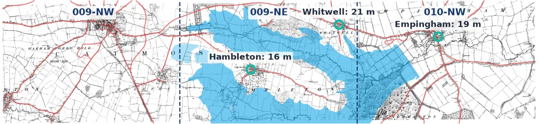
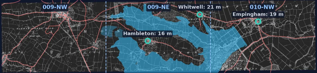
Three sheets, one grid, no seams — and the two placed only from the layout land within about 20 m of their churches, the same accuracy as the sheet that had control points:
Check the crops, compute corners, verify on unused features
1. Confirm the scans are cropped at the sheet lines
The method depends on the scan's edges being the sheet's edges. A six-inch quarter sheet covers 3 by 2 miles; the fitted scale of 009-NW says whether the scan matches:
A = fit_affine(GCPS)
m_per_px = np.hypot(*A[1]), np.hypot(*A[2])
w, h = Image.open("data/os_009-NW.jpg").size
print(f"009-NW: {w} x {h} px = {w * m_per_px[0] / 1609.344:.3f} x {h * m_per_px[1] / 1609.344:.3f} miles")
for name in SHEETS[1:]:
    print(name, Image.open(f"data/os_{name}.jpg").size)
009-NW: 5343 x 3573 px = 2.997 x 1.999 miles
009-NE (5396, 3590)
010-NW (5395, 3589)
Three miles by two, to within a few thousandths. The neighbours' scans are a few dozen pixels larger — scanned at a slightly different resolution — so each gets its own pixel size, but the same ground size.
2. Compute the neighbours' corners
Sheet 009-NE is the next three miles east of 009-NW, on the same grid and at the same rotation; 010-NW is three miles further. In 009-NW's pixel frame, a neighbour's corners are just offset by whole sheet widths:
for name in SHEETS[1:]:
    print(name, [(round(e), round(n)) for _, _, e, n in corner_gcps(name)][:2], "...")
009-NE [(488052, 309370), (492876, 309410)] ...
010-NW [(492876, 309410), (497699, 309451)] ...
This extrapolates 009-NW's fit up to ten kilometres east, so any error in its scale or rotation grows with distance. That is the thing to check.
3. Check against features you did not use
Three churches on the neighbouring sheets — Whitwell, Hambleton and Empingham — were located on the scans by eye and compared with OpenStreetMap:
for label, name, c, r, e, n in CHURCHES:
    g = corner_gcps(name)
    A_n = fit_affine([(None, cc, rr, ee, nn) for cc, rr, ee, nn in g])
    x, y = np.array([1, c, r]) @ A_n
    print(f"{label:22} on {name}: {np.hypot(x - e, y - n):5.1f} m from OpenStreetMap")
Whitwell, St Michael on 009-NE: 20.9 m from OpenStreetMap
Hambleton, St Andrew on 009-NE: 16.1 m from OpenStreetMap
Empingham, St Peter on 010-NW: 19.0 m from OpenStreetMap
All three are within the 8–22 m leave-one-out range of the sheet that had control points. Ten kilometres of extrapolation added nothing measurable, which says the scans' edges really are the sheet lines and the series really is on one grid.
4. Warp onto one aligned grid
targetAlignedPixels=True snaps every output's corners to whole multiples of the resolution, so the three rasters share one pixel grid and a mosaic never resamples them again:
for name in SHEETS:
    gt = gdal.Open(f"data/{name}_bng.tif").GetGeoTransform()
    print(name, "origin", gt[0], gt[3], "- whole metres:", gt[0] % 1 == 0 and gt[3] % 1 == 0)
009-NW origin 483228.0 309370.0 - whole metres: True
009-NE origin 488052.0 309411.0 - whole metres: True
010-NW origin 492875.0 309451.0 - whole metres: True
5. Mosaic and check the seams
gdal.BuildVRT mosaics without copying pixels. At a seam, the alpha bands show whether the sheets meet, overlap, or leave a gap:
mos = gdal.Open("data/mosaic.vrt")
alpha = mos.GetRasterBand(2).ReadAsArray()
gt = mos.GetGeoTransform()
for name in SHEETS[1:]:
    col = int(round((corner_gcps(name)[0][2] - gt[0]) / gt[1]))
    rows = slice(300, alpha.shape[0] - 300)                    # away from the rotated top and bottom edges
    gap = (alpha[rows, col - 3:col + 3] == 0).sum()
    print(f"seam at {name}: {gap} transparent pixels in a 6-pixel strip")
seam at 009-NE: 0 transparent pixels in a 6-pixel strip
seam at 010-NW: 0 transparent pixels in a 6-pixel strip
No gaps: the sheets meet edge to edge. Where two warps do overlap by a pixel, the VRT takes the later file; with a shared grid and matching corners there is nothing to blend.
Joining three Rutland sheets into one COG
The data used on this page
Ordnance Survey six-inch sheets Rutland 009-NW, 009-NE and 010-NW (1884–1891) from Wikimedia Commons (public domain); OpenStreetMap from Geofabrik (1 January 2026; © OpenStreetMap contributors, ODbL) for the control points and the check churches.
from pathlib import Path

import numpy as np
import requests
from osgeo import gdal
from PIL import Image

gdal.UseExceptions()
Path("data").mkdir(exist_ok=True)
UA = {"User-Agent": "spatialworkflow.io guide (https://www.spatialworkflow.io)"}
COMMONS = "https://upload.wikimedia.org/wikipedia/commons/"
URLS = {
    "009-NW": COMMONS + "a/a0/Map_of_Rutland_OS_Map_name_009-NW%2C_Ordnance_Survey%2C_1884-1891.jpg",
    "009-NE": COMMONS + "8/80/Map_of_Rutland_OS_Map_name_009-NE%2C_Ordnance_Survey%2C_1884-1891.jpg",
    "010-NW": COMMONS + "4/47/Map_of_Rutland_OS_Map_name_010-NW%2C_Ordnance_Survey%2C_1884-1891.jpg",
}
SHEETS = list(URLS)
for name, url in URLS.items():
    if not Path(f"data/os_{name}.jpg").exists():
        Path(f"data/os_{name}.jpg").write_bytes(requests.get(url, headers=UA, timeout=300).content)

GCPS = [  # (id, pixel, line, easting, northing) on 009-NW
    ("oakham_church",          3141,  487, 486065.6, 308906.1),
    ("egleton_church",         4824, 2031, 487598.5, 307540.3),
    ("brooke_rd_crossing",     2956, 1159, 485892.0, 308306.8),
    ("egleton_level_crossing", 3998, 2481, 486838.1, 307119.0),
    ("stamford_rd_guide_post", 5127,  988, 487872.3, 308486.1),
    ("braunston_rd_bridleway", 1263, 1675, 484382.4, 307839.2),
    ("brooke_guide_post",      1547, 3292, 484648.2, 306376.1),
]
SHEET_OFFSET = {"009-NW": (0, 0), "009-NE": (1, 0), "010-NW": (2, 0)}   # sheet widths east, heights south
CHURCHES = [  # (label, sheet, column, row of the church symbol, OSM easting, northing)
    ("Whitwell, St Michael", "009-NE", 4808,  685, 492369.5, 308805.8),
    ("Hambleton, St Andrew", "009-NE", 2140, 2027, 489966.1, 307582.4),
    ("Empingham, St Peter",  "010-NW", 2440, 1088, 495070.2, 308471.1),
]

def fit_affine(points):
    X = np.array([[1, g[1], g[2]] for g in points], float)
    return np.linalg.lstsq(X, np.array([[g[3], g[4]] for g in points]), rcond=None)[0]

def corner_gcps(name):
    """(column, row, easting, northing) at the four corners of a sheet, from 009-NW's fit and the layout."""
    A = fit_affine(GCPS)
    w0, h0 = Image.open("data/os_009-NW.jpg").size
    w, h = Image.open(f"data/os_{name}.jpg").size
    dx, dy = SHEET_OFFSET[name]
    return [(c, r, *(np.array([1, dx * w0 + c * w0 / w, dy * h0 + r * h0 / h]) @ A))
            for c, r in ((0, 0), (w, 0), (w, h), (0, h))]

print({n: Path(f"data/os_{n}.jpg").stat().st_size for n in SHEETS})
{'009-NW': 2653911, '009-NE': 3057362, '010-NW': 3474375}
Example 1: what a badly trimmed scan does
The layout assumes each scan starts exactly at its sheet line. Pretend 009-NE had lost a 50-pixel strip from its left edge — a margin trimmed carelessly — and the check churches move with it:
def corner_gcps_trimmed(name, lost_left):
    w, h = Image.open(f"data/os_{name}.jpg").size
    A = fit_affine(GCPS)
    w0, h0 = Image.open("data/os_009-NW.jpg").size
    dx, dy = SHEET_OFFSET[name]
    # the scan now starts lost_left pixels into the sheet, but is still treated as the whole sheet
    return [(c, r, *(np.array([1, dx * w0 + c * w0 / (w - lost_left), dy * h0 + r * h0 / h]) @ A))
            for c, r in ((0, 0), (w - lost_left, 0), (w - lost_left, h), (0, h))]

for lost in (0, 50):
    for label, name, c, r, e, n in CHURCHES[:2]:
        A_n = fit_affine([(None, cc, rr, ee, nn) for cc, rr, ee, nn in corner_gcps_trimmed(name, lost)])
        x, y = np.array([1, c - lost, r]) @ A_n
        print(f"{lost:2} px trimmed  {label:22} {np.hypot(x - e, y - n):5.1f} m")
0 px trimmed Whitwell, St Michael 20.9 m
0 px trimmed Hambleton, St Andrew 16.1 m
50 px trimmed Whitwell, St Michael 24.9 m
50 px trimmed Hambleton, St Andrew 21.9 m
The layout stretches what is left of the scan to fill the whole sheet, so the error is largest at the trimmed edge — the full 50 pixels, about 45 m — and falls to nothing at the opposite one. Hambleton, near the middle, moved 6 m; Whitwell, near the right edge, 4 m. A feature near the left edge would be 45 m out with nothing to show for it, which is why step 1 measures each scan against the sheet size before trusting the layout.
Example 2: write the mosaic as one Cloud-Optimised GeoTIFF
A VRT is a set of references; to share the mosaic, write it out:
gdal.Translate("data/rutland_009nw_010nw.tif", "data/mosaic.vrt", format="COG",
               creationOptions=["COMPRESS=DEFLATE", "PREDICTOR=2", "OVERVIEWS=AUTO"])
info = gdal.Info("data/rutland_009nw_010nw.tif", format="json")
print(info["size"], len(info["bands"][0].get("overviews", [])), "overview levels,",
      round(Path("data/rutland_009nw_010nw.tif").stat().st_size / 1e6, 1), "MB")
[14491, 3339] 5 overview levels, 24.3 MB
A series is one map cut into sheets
A map series is a single map cut into sheets. The Ordnance Survey's county series six-inch sheets were drawn on a projection centred on a county origin, with sheet lines at fixed intervals, so every sheet's corners sit at known positions in the same coordinate system. The modern scans preserve that wherever they are trimmed to the sheet lines — which is what step 1 checks.
That turns the georeferencing of a series into one fit and a lookup. The sheet with the best control points fixes the series' scale, rotation and position in the modern grid; every other sheet inherits them by position. Errors that would have been independent and uncorrelated across sheets — and visible as steps at every join — become one systematic error shared by all, which is invisible at the joins and can be measured once, against features on any sheet.
Two caveats keep it honest. First, the county series used a separate origin for each county or group of counties, so the layout holds within Rutland's series but not across a county boundary; a Leicestershire sheet needs its own anchor. Second, paper shrinks: each sheet's own distortion, a few metres here, is not in the layout and remains as local error. The check churches measure both together.
Scan edges, mixed resolutions and VRT order
- Check the scan edges. A scan with a margin or a trimmed edge breaks the layout; measure it against 3 × 2 miles first.
- Different scan resolutions are fine; give each sheet its own pixel size.
- One county series, one grid. Neighbours across a county boundary need their own control points.
- Align the output grids with
targetAlignedPixels, or the mosaic resamples a second time. - BuildVRT takes the last file where sheets overlap; order the list deliberately.
- Check with independent features on every sheet you place by layout.
Internal links
- How to georeference a scanned map with GDAL — the single-sheet version
- How to measure change from an old map — the Hambleton valley under Rutland Water, on these sheets
- How to overlay a georeferenced old map on a web map — tiling the mosaic
- How to download scanned historical maps — all thirty Rutland quarter sheets
- Ground control points explained — why two points cannot fix a sheet
FAQ
How do I mosaic georeferenced map sheets?
Warp each sheet to the same CRS and resolution with targetAlignedPixels=True and an alpha band, then combine them with gdal.BuildVRT; write a single file with gdal.Translate.
Do I need control points on every sheet?
Not for a series cropped at its sheet lines. Fit one sheet well, compute its neighbours' corners from the sheet layout, and check them against a few independent features.
Why are there steps at the joins between my sheets?
Each sheet was georeferenced independently and the fits disagree along the shared edge. Placing neighbours from one fit and the sheet layout removes the disagreement.
How big is a six-inch quarter sheet?
Three miles by two — about 4.83 by 3.22 km — at a scale of six inches to the mile (1:10,560).