
Old Map Projections Explained: What Grid Was a Historical Map Drawn On?
On this page
Problem statement
Every flat map is drawn on some projection, and an old map's projection decides how it should be georeferenced. If it was drawn on a known projection with known sheet lines, its corners can be computed and its geometry restored exactly; if it was compiled by eye from travellers' distances, there is no projection to recover and the best you can do is a fitted transformation. Treating the first kind like the second throws information away; treating the second like the first invents precision.
This page tests both kinds on real maps of Rutland. The Ordnance Survey six-inch sheets of 1884–1891 belong to the County Series, drawn on a Cassini projection centred on a meridian through Dunnose on the Isle of Wight; John Speed's county map of 1611 was not drawn on any projection in the modern sense. The georeferenced sheets themselves show which is which.
Quick answer
Put the georeferenced sheet corners into the projection the series is supposed to use and check whether they fall on the sheet lines. For the County Series that is Cassini on the Dunnose meridian, with quarter sheets 3 miles wide:
for name in SHEETS:
    e, n = corner_bng(name)                                   # top-left corner from the georeferencing
    x_ft, y_ft = [v / FOOT for v in to_cassini.transform(e, n)]
    print(f"{name}: {x_ft:9,.0f} ft east of the Dunnose meridian = {x_ft / 15840:6.3f} x 3 miles")
009-NW: 95,051 ft east of the Dunnose meridian = 6.001 x 3 miles
009-NE: 110,882 ft east of the Dunnose meridian = 7.000 x 3 miles
010-NW: 126,713 ft east of the Dunnose meridian = 8.000 x 3 miles
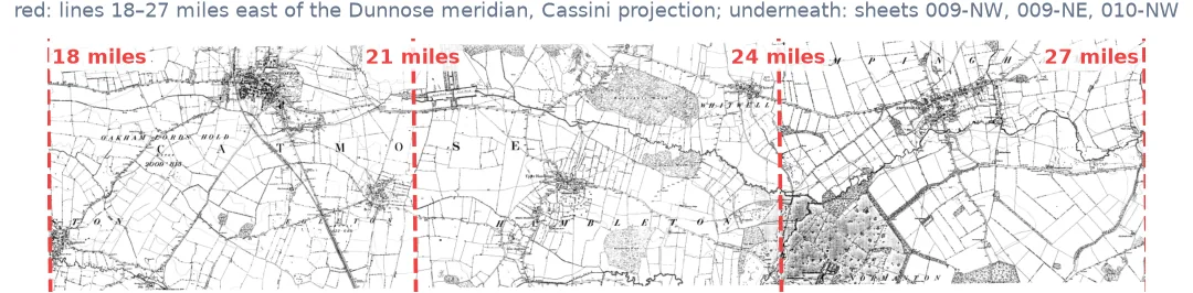
The western edges of three adjacent sheets sit within a few feet of whole multiples of three miles from the meridian — six, seven and eight sheet-widths east of it — so the County Series geometry is recovered from nothing more than seven control points on one sheet:
Find the series' projection, check sheet lines
1. Find out what the series used
The projection is a historical fact, not something to guess. For the County Series the National Library of Scotland's notes on the six-inch maps record that Rutland was one of the central English counties drawn on the Dunnose meridian, a Cassini projection whose central meridian passes through Dunnose on the Isle of Wight, 1°11′50.136″ W, 50°37′03.748″ N:
op = DUNNOSE.source_crs.coordinate_operation
print(op.method_name, "on", DUNNOSE.ellipsoid.name)
print({p.name: round(p.value, 6) for p in op.params})
Cassini-Soldner on Airy 1830
{'Latitude of natural origin': 50.617708, 'Longitude of natural origin': -1.19726, 'False easting': 0.0, 'False northing': 0.0}
The ellipsoid is Airy 1830, the one the National Grid still uses; the datum shift to OSGB 1936 here uses its usual seven parameters, which is close enough for a test at the scale of feet.
2. Check the sheet lines
Quarter sheets of the six-inch County Series are 3 miles east–west and 2 miles north–south. If the georeferenced corners fall on multiples of those distances from the meridian, the georeferencing and the projection agree:
for name in SHEETS:
    e, n = corner_bng(name)
    x_ft, y_ft = [v / FOOT for v in to_cassini.transform(e, n)]
    print(f"{name}: east {x_ft % 15840:7.0f} ft past a 3-mile line;  north {y_ft % 10560:7.0f} ft past a 2-mile line")
009-NW: east 11 ft past a 3-mile line; north 1405 ft past a 2-mile line
009-NE: east 2 ft past a 3-mile line; north 1361 ft past a 2-mile line
010-NW: east 15833 ft past a 3-mile line; north 1317 ft past a 2-mile line
East–west, within a few feet. North–south the corners do not fall on 2-mile multiples counted from Dunnose's latitude; the rows of County Series sheets were evidently laid out from a different starting line, which this test cannot identify. The east–west agreement is the striking result: it is what a Cassini grid predicts and an arbitrary fit does not.
3. See what the projection does to the National Grid
The Cassini grid and the National Grid are both transverse projections of the same ellipsoid, on different central meridians: Dunnose, 1.2° W, and the National Grid's 2° W. At Oakham their north directions differ:
e, n = 486065.6, 308906.1
x, y = to_cassini.transform(e, n)
a, b = np.array(from_cassini.transform(x, y)), np.array(from_cassini.transform(x, y + 1000))
print(f"County Series north points {np.degrees(np.arctan2(*(b - a))):+.2f} deg from National Grid north at Oakham; "
      f"1 km of Cassini = {np.hypot(*(b - a)):.2f} m of National Grid")
County Series north points -0.64 deg from National Grid north at Oakham; 1 km of Cassini = 999.66 m of National Grid
That is the rotation every georeferenced six-inch sheet of Rutland shows. The affine fit to seven control points measured about half a degree; the projection says 0.64°. The difference, 0.16° across a 4.8 km sheet, is about 13 m at its edge — inside the control points' error, and the reason the corner tests in step 2 drift by a few dozen feet from sheet to sheet.
4. Test a map that had no projection
Speed's map has no sheet lines to test, so test its distortion instead. A map drawn on a projection has smooth, predictable distortion; a compiled map has local, irregular error. The leave-one-out errors of the early county map guide show which:
for order in (1, 2):
    X = design(SPEED, order)
    W = np.array([[g[3], g[4]] for g in SPEED])
    lo = [np.hypot(*(X[i] @ np.linalg.lstsq(np.delete(X, i, 0), np.delete(W, i, 0), rcond=None)[0] - W[i]))
          for i in range(len(SPEED))]
    print(f"Speed, polynomial order {order}: leave-one-out RMS {np.sqrt(np.mean(np.square(lo))):5.0f} m")
Speed, polynomial order 1: leave-one-out RMS 695 m
Speed, polynomial order 2: leave-one-out RMS 549 m
A smooth transformation removes about a fifth of the error; the rest is village by village. That is the signature of a compiled map: no projection, or none that survives the compilation, to recover.
Sheet corners from the Cassini projection alone
The data used on this page
Ordnance Survey six-inch sheets Rutland 009-NW, 009-NE and 010-NW (1884–1891) and John Speed's Rutlandshire (1676 edition of the 1611 map, David Rumsey Map Collection, Stanford Libraries), all from Wikimedia Commons (public domain); OpenStreetMap from Geofabrik (1 January 2026; © OpenStreetMap contributors, ODbL). The Dunnose origin is from the National Library of Scotland's notes on the six-inch County Series.
from pathlib import Path

import geopandas as gpd
import numpy as np
import requests
from PIL import Image
from pyproj import CRS, Proj, Transformer

Path("data").mkdir(exist_ok=True)
UA = {"User-Agent": "spatialworkflow.io guide (https://www.spatialworkflow.io)"}
COMMONS = "https://upload.wikimedia.org/wikipedia/commons/"
for name, path in {"009-NW": "a/a0/", "009-NE": "8/80/", "010-NW": "4/47/"}.items():
    if not Path(f"data/os_{name}.jpg").exists():
        url = f"{COMMONS}{path}Map_of_Rutland_OS_Map_name_{name}%2C_Ordnance_Survey%2C_1884-1891.jpg"
        Path(f"data/os_{name}.jpg").write_bytes(requests.get(url, headers=UA, timeout=300).content)
if not Path("data/rutland.shp.zip").exists():
    Path("data/rutland.shp.zip").write_bytes(requests.get(
        "https://download.geofabrik.de/europe/united-kingdom/england/rutland-260101-free.shp.zip",
        headers=UA, timeout=300).content)

GCPS = [  # (id, pixel, line, easting, northing) on 009-NW
    ("oakham_church",          3141,  487, 486065.6, 308906.1),
    ("egleton_church",         4824, 2031, 487598.5, 307540.3),
    ("brooke_rd_crossing",     2956, 1159, 485892.0, 308306.8),
    ("egleton_level_crossing", 3998, 2481, 486838.1, 307119.0),
    ("stamford_rd_guide_post", 5127,  988, 487872.3, 308486.1),
    ("braunston_rd_bridleway", 1263, 1675, 484382.4, 307839.2),
    ("brooke_guide_post",      1547, 3292, 484648.2, 306376.1),
]
SHEETS = {"009-NW": 0, "009-NE": 1, "010-NW": 2}            # sheet widths east of 009-NW
DUNNOSE = CRS.from_proj4("+proj=cass +lat_0=50.617708 +lon_0=-1.197260 +x_0=0 +y_0=0 +ellps=airy "
                         "+towgs84=446.448,-125.157,542.06,0.15,0.247,0.842,-20.489 +units=m +no_defs")
to_cassini = Transformer.from_crs(27700, DUNNOSE, always_xy=True)
from_cassini = Transformer.from_crs(DUNNOSE, 27700, always_xy=True)
FOOT = 0.3048
to_ll = Transformer.from_crs(27700, 4326, always_xy=True)

X = np.array([[1, g[1], g[2]] for g in GCPS], float)
A = np.linalg.lstsq(X, np.array([[g[3], g[4]] for g in GCPS]), rcond=None)[0]
W0 = Image.open("data/os_009-NW.jpg").size[0]

def corner_bng(name):
    """Top-left corner of a sheet in British National Grid, from 009-NW's fit and the sheet layout."""
    return tuple(np.array([1, SHEETS[name] * W0, 0]) @ A)

SPEED_PX = {  # modern village name: (column, row) of Speed's church symbol
    "Oakham": (4960, 4035), "Langham": (4475, 3725), "Barleythorpe": (4755, 3920), "Egleton": (5265, 4290),
    "Braunston in Rutland": (4470, 4745), "Brooke": (4705, 4790), "Gunthorpe": (5095, 4745), "Manton": (5430, 4935),
    "Greetham": (6200, 2930), "Cottesmore": (5715, 3205), "Exton": (6165, 3500), "Empingham": (6730, 3890),
    "Whitwell": (6245, 4080), "Upper Hambleton": (5795, 4285), "Burley on the Hill": (5490, 3705), "Barrow": (5495, 2965),
    "Pickworth": (7375, 2930), "Tickencote": (7595, 3875), "Lyndon": (6005, 4880), "Edith Weston": (6415, 4555),
    "Wing": (5735, 5245), "Pilton": (6315, 5335), "North Luffenham": (6600, 5110), "South Luffenham": (6705, 5400),
    "Ridlington": (4755, 5425), "Preston": (5335, 5380), "Glaston": (5650, 5690), "Morcott": (6465, 5735),
    "Ayston": (4960, 5765), "Uppingham": (5125, 6080), "Bisbrooke": (5605, 6035), "Seaton": (5960, 6430),
    "Barrowden": (7070, 5985),
}
places = gpd.read_file("/vsizip/data/rutland.shp.zip/gis_osm_places_free_1.shp").to_crs(27700)
places = places[places.fclass.isin(["village", "town", "hamlet"])].drop_duplicates("name").set_index("name")
SPEED = [(k, c, r, places.loc[k].geometry.x, places.loc[k].geometry.y) for k, (c, r) in SPEED_PX.items()]

def design(points, order):
    c = np.array([g[1] for g in points], float) / 1e4
    r = np.array([g[2] for g in points], float) / 1e4
    cols = [np.ones_like(c), c, r] + ([c * c, c * r, r * r] if order == 2 else [])
    return np.column_stack(cols)

print([round(v) for v in corner_bng("009-NW")])
[483228, 309330]
Example 1: compute a sheet's corners from the projection alone
If the County Series grid is right, a sheet's corners can be computed without any control points at all — from the meridian, the sheet size, and which sheet it is. Taking the nearest 3-mile line to 009-NW's western edge, and the northing the georeferencing gave:
e, n = corner_bng("009-NW")
x, y = to_cassini.transform(e, n)
x_line = round(x / FOOT / 15840) * 15840 * FOOT                        # the 3-mile sheet line
predicted = [from_cassini.transform(x_line + dx * 15840 * FOOT, y - dy * 10560 * FOOT) for dx, dy in ((0, 0), (1, 0), (1, 1), (0, 1))]
fitted = [tuple(np.array([1, c, r]) @ A) for c, r in ((0, 0), (5343, 0), (5343, 3573), (0, 3573))]
for (pe, pn), (fe, fn) in zip(predicted, fitted):
    print(f"projection {pe:10.1f} {pn:10.1f}   control points {fe:10.1f} {fn:10.1f}   apart {np.hypot(pe - fe, pn - fn):5.1f} m")
projection 483224.9 309329.6 control points 483228.1 309329.6 apart 3.2 m
projection 488051.1 309383.4 control points 488051.8 309370.1 apart 13.4 m
projection 488086.9 306166.0 control points 488071.2 306152.9 apart 20.5 m
projection 483260.8 306112.2 control points 483247.5 306112.4 apart 13.3 m
Corners from the projection and corners from seven hand-picked control points agree to within the control points' own error. On a sheet with no surviving features to use as control points, the projection alone would place it.
Example 2: the scale of the Cassini grid
Cassini keeps scale true along the central meridian; away from it, distances north–south on the map are stretched, increasingly with distance east or west. pyproj reports the projection's own scale factors at any point:
proj = Proj(DUNNOSE.source_crs)
for name in SHEETS:
    lon, lat = to_ll.transform(*corner_bng(name))
    f = proj.get_factors(lon, lat)
    x, _ = to_cassini.transform(*corner_bng(name))
    print(f"{name}: {x / 1000:5.1f} km east of the meridian; north-south scale {f.meridional_scale:.7f} "
          f"= {(f.meridional_scale - 1) * 1e6:4.1f} mm per km")
009-NW: 29.0 km east of the meridian; north-south scale 1.0000102 = 10.2 mm per km
009-NE: 33.8 km east of the meridian; north-south scale 1.0000139 = 13.9 mm per km
010-NW: 38.6 km east of the meridian; north-south scale 1.0000182 = 18.2 mm per km
A centimetre or two per kilometre — invisible at six inches to the mile. Counties far from their meridian had larger errors, because the stretch grows with the square of the distance; that is one reason the National Grid replaced the County Series' many origins with one.
A projection is a rule
A projection is the rule that turns positions on the curved Earth into positions on flat paper. Any systematically surveyed map has one, chosen by the surveyors and applied consistently; maps compiled from earlier maps and descriptions inherit whatever their sources had, blurred by the compilation, and often end up with no consistent projection at all.
The Ordnance Survey's County Series used the Cassini projection, which places the paper along a central meridian and measures distances east or west of it along great circles. Each group of counties had its own meridian to keep the distortion small — Rutland's is Dunnose's, shared with much of central and southern England. Sheet lines were drawn at fixed distances from that meridian, so a sheet's position is a matter of arithmetic once the meridian is known. The test in step 2 recovers that arithmetic from a georeferenced scan, to within a few feet.
The National Grid, from the 1930s, uses a Transverse Mercator projection on a single meridian at 2° W for the whole country. Converting between the two is not just a shift: the two grids' north directions differ by an amount that depends on where you are, about two-thirds of a degree at Oakham — the rotation every affine fit to a Rutland six-inch sheet picks up.
A compiled map like Speed's is different in kind. Its geometry is the sum of many local judgements, and its errors are local. There is no projection to put it on; the honest approach is the empirical one — a fitted transformation, a leave-one-out error, and a distortion grid to show where the map is good and where it is not.
County meridians, datums and old feet
- Look up the projection; county origins and sheet systems are documented for the County Series.
- Several counties shared a meridian, so sheets join across those county boundaries but not across others.
- North–south sheet lines did not test cleanly here; a test that fails is information, not something to fit away.
- Datum shifts at the scale of feet need care; the seven-parameter transformation used here is good to a few metres.
- Old foot definitions differ by parts per million; irrelevant at six inches to the mile.
- No projection is a valid answer for compiled maps; do not invent one.
Internal links
- How to mosaic historical map sheets — the sheet layout used in practice
- Georeferencing explained — fitting when no projection is known
- How accurate is a historical map? — surveyed against compiled
- How to georeference an early county map — Speed, empirically
- How to draw a distortion grid on an old map — showing a compiled map's errors
FAQ
What projection did the Ordnance Survey County Series use?
The Cassini projection, on a set of county origins. Rutland's six-inch and 1:2500 sheets used the Dunnose meridian on the Isle of Wight, shared with much of central and southern England.
How can I tell whether an old map has a projection?
Check the documentation for the series first. Empirically, a surveyed map on a known projection has smooth distortion and sheet corners that fall on regular lines in that projection; a compiled map has local, irregular errors that no smooth transformation removes.
Why is my georeferenced six-inch sheet rotated against the National Grid?
The County Series grid and the National Grid have different central meridians, so their north directions differ — by about 0.64° at Oakham.
Did John Speed use a map projection?
Not in a form that can be recovered from his map of Rutland: its errors are village by village, and a smooth transformation removes only about a fifth of them.