How Accurate Is a Historical Map? Measuring Survey Error

Problem statement

An old map overlaid on modern data always looks a little off, and the question that matters is how much of that is the map. A georeferenced map can never be more accurate than the survey behind it: if the surveyor put a village 700 m from where it stands, no choice of control points or transformation will move it back. Before measuring change from an old map — a river that shifted, a wood that shrank — you need a number for how wrong the map itself is.

This page measures it for two maps of the same county drawn 270 years apart: John Speed's Rutland, first published in 1611 (here in the 1676 edition), and the Ordnance Survey six-inch sheet of Oakham, surveyed 1884–1891.

Quick answer

Fit an affine transformation to points identified on the map and in modern data, predict each point from the others, and take the root-mean-square of the misses. That number is the map's positional accuracy as you can use it:

for label, pts in (("Speed, 1611 (1676 ed.)", SPEED), ("OS six-inch, 1884-91", OS)):
    err = np.hypot(*loo_affine(pts).T)
    print(f"{label:24} {len(pts):2} points   leave-one-out RMS {rms(err):6.1f} m   worst {err.max():6.1f} m")

Speed, 1611 (1676 ed.)   33 points   leave-one-out RMS  695.0 m   worst 1423.3 m
OS six-inch, 1884-91      7 points   leave-one-out RMS   17.5 m   worst   22.2 m

Speed's villages are typically 700 m out and up to 1.4 km; the Victorian survey is within about 20 m. At the same scale, one map's errors are visible arrows and the other's are invisible:

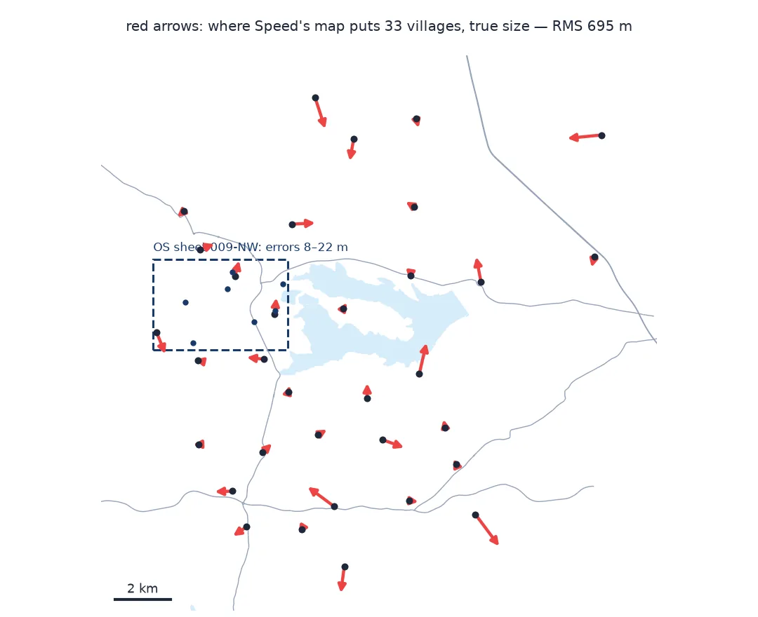
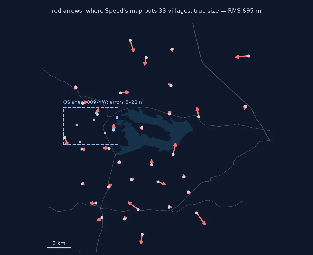
Shared points, an overall fit, leave-one-out predictions

1. Choose points that both maps and today agree on

Accuracy can only be measured where you can identify the same thing on the old map and in modern data. For Speed that is the church symbol he drew for each village, matched to OpenStreetMap's point for the village; for the six-inch sheet, the churches, crossings and guide posts picked in the control-point guide:

print("Speed points:", ", ".join(g[0] for g in SPEED[:8]), "...", len(SPEED), "in all")
print("OS points:   ", ", ".join(g[0] for g in OS))

Speed points: Oakham, Langham, Barleythorpe, Egleton, Braunston in Rutland, Brooke, Gunthorpe, Manton ... 33 in all
OS points:    oakham_church, egleton_church, brooke_rd_crossing, egleton_level_crossing, stamford_rd_guide_post, braunston_rd_bridleway, brooke_guide_post

A village point in OpenStreetMap is placed somewhere near the centre of the village, not on the church, so the Speed comparison carries an extra uncertainty of perhaps a hundred metres. Against errors of 700 m that does not change the conclusion; against errors of 20 m it would, which is why the OS points are individual features.

2. Fit the map's overall geometry

An affine transformation takes out everything that is a property of the sheet rather than of the survey — the scale, the rotation of the paper, any shear — and leaves what is left as error:

for label, pts in (("Speed", SPEED), ("OS", OS)):
    X = np.array([[1, g[1], g[2]] for g in pts], float)
    W = np.array([[g[3], g[4]] for g in pts], float)
    c = np.linalg.lstsq(X, W, rcond=None)[0]
    (a, d), (b, e) = c[1], c[2]
    print(f"{label:6} {np.hypot(a, d):.3f} m per pixel; north on the sheet is {np.degrees(np.arctan2(d, a)):+.2f} deg from grid north")

Speed  4.799 m per pixel; north on the sheet is -4.00 deg from grid north
OS     0.903 m per pixel; north on the sheet is +0.48 deg from grid north

Speed's sheet is turned four degrees: his "north" is not quite the National Grid's, which is a property of how the map was compiled, not an error at any village. The affine fit removes it, as it should.

3. Predict each point from the others

Residuals from a fit that includes a point understate its error. Leaving each point out gives an honest estimate:

sp = pd.Series(np.hypot(*loo_affine(SPEED).T), index=[g[0] for g in SPEED]).round()
print(sp.sort_values(ascending=False).head(6).to_string())
print(f"median {sp.median():.0f} m; {(sp > 1000).sum()} of {len(sp)} villages more than 1 km out")

Barrowden       1423.0
Pickworth       1224.0
Barrow          1192.0
Glaston         1177.0
Edith Weston    1144.0
Seaton           962.0
median 561 m; 5 of 33 villages more than 1 km out

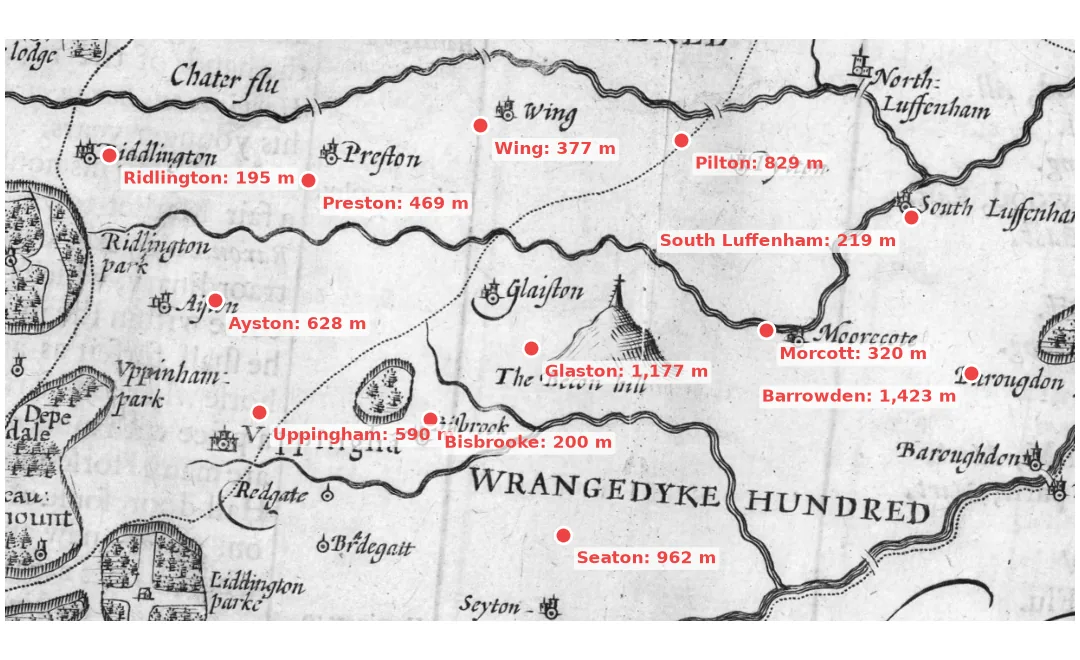
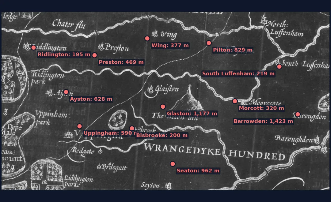
The worst are not random: Barrowden, Seaton and Glaston sit near the county's southern edge, Barrow and Pickworth near its northern one, where Speed had fewest neighbours to place them against.

4. Look for pattern in the errors

Random errors point every way. Systematic ones — a stretched quarter of the county, a misplaced river — point together:

v = loo_affine(SPEED)
E = np.array([g[3] for g in SPEED]); N = np.array([g[4] for g in SPEED])
print("correlation of east error with easting:", round(np.corrcoef(E, v[:, 0])[0, 1], 2),
      "| north error with northing:", round(np.corrcoef(N, v[:, 1])[0, 1], 2))

correlation of east error with easting: -0.12 | north error with northing: -0.1

Neither correlation is large, so the errors are not a simple stretch an affine fit has missed. A second-order polynomial — which 33 points can support, unlike the seven on the OS sheet — tests for smooth bowing:

def loo_poly2(points):
    X = np.array([[1, c, r, c * c, c * r, r * r] for _, c, r, _, _ in points], float) / [1, 1e4, 1e4, 1e8, 1e8, 1e8]
    W = np.array([[g[3], g[4]] for g in points], float)
    return np.array([X[i] @ np.linalg.lstsq(np.delete(X, i, 0), np.delete(W, i, 0), rcond=None)[0] - W[i]
                     for i in range(len(points))])

print(f"Speed, leave-one-out RMS: affine {rms(np.hypot(*loo_affine(SPEED).T)):.0f} m, "
      f"polynomial 2 {rms(np.hypot(*loo_poly2(SPEED).T)):.0f} m")

Speed, leave-one-out RMS: affine 695 m, polynomial 2 549 m

About a fifth of Speed's error is a smooth distortion of the county, and the polynomial takes it out, from 695 m to 549 m. Most is not: what remains is village by village, which is what a map compiled from travelled distances and local knowledge looks like, and no smooth transformation can remove it.

5. Turn the number into a rule

The leave-one-out RMS sets the smallest change the map can show. With 695 m on Speed's map, a village "moving" 300 m between Speed and today is noise; on the six-inch sheet, a field boundary that moved 50 m is very probably real.

Speed's villages against the Ordnance Survey

The data used on this page

John Speed's Rutlandshire from the 1676 Bassett & Chiswell edition of The Theatre of the Empire of Great Britaine, scanned by the David Rumsey Map Collection, David Rumsey Map Center, Stanford Libraries, via Wikimedia Commons (public domain); the Ordnance Survey six-inch sheet Rutland 009-NW (1884–1891, Wikimedia Commons, public domain); OpenStreetMap from Geofabrik (1 January 2026; © OpenStreetMap contributors, ODbL). The church symbols on Speed's map were located by eye at full resolution.

from pathlib import Path

import geopandas as gpd
import numpy as np
import pandas as pd
import requests

Path("data").mkdir(exist_ok=True)
UA = {"User-Agent": "spatialworkflow.io guide (https://www.spatialworkflow.io)"}
downloads = {
    "data/speed_rutland.jpg": "https://upload.wikimedia.org/wikipedia/commons/9/9c/Rutlandshire._%28insets%29_Oukham."
                              "_Stanford._%28IA_dr_rutlandshire-insets-oukham-stanford-12058072%29.jpg",
    "data/rutland.shp.zip": "https://download.geofabrik.de/europe/united-kingdom/england/rutland-260101-free.shp.zip",
}
for target, url in downloads.items():
    if not Path(target).exists():
        Path(target).write_bytes(requests.get(url, headers=UA, timeout=600).content)

SPEED_PX = {  # OSM village name: (column, row) of the church symbol on Speed's sheet
    "Oakham": (4960, 4035), "Langham": (4475, 3725), "Barleythorpe": (4755, 3920), "Egleton": (5265, 4290),
    "Braunston in Rutland": (4470, 4745), "Brooke": (4705, 4790), "Gunthorpe": (5095, 4745), "Manton": (5430, 4935),
    "Greetham": (6200, 2930), "Cottesmore": (5715, 3205), "Exton": (6165, 3500), "Empingham": (6730, 3890),
    "Whitwell": (6245, 4080), "Upper Hambleton": (5795, 4285), "Burley on the Hill": (5490, 3705), "Barrow": (5495, 2965),
    "Pickworth": (7375, 2930), "Tickencote": (7595, 3875), "Lyndon": (6005, 4880), "Edith Weston": (6415, 4555),
    "Wing": (5735, 5245), "Pilton": (6315, 5335), "North Luffenham": (6600, 5110), "South Luffenham": (6705, 5400),
    "Ridlington": (4755, 5425), "Preston": (5335, 5380), "Glaston": (5650, 5690), "Morcott": (6465, 5735),
    "Ayston": (4960, 5765), "Uppingham": (5125, 6080), "Bisbrooke": (5605, 6035), "Seaton": (5960, 6430),
    "Barrowden": (7070, 5985),
}
places = gpd.read_file("/vsizip/data/rutland.shp.zip/gis_osm_places_free_1.shp").to_crs(27700)
places = places[places.fclass.isin(["village", "town", "hamlet"])].drop_duplicates("name").set_index("name")
SPEED = [(k, c, r, places.loc[k].geometry.x, places.loc[k].geometry.y) for k, (c, r) in SPEED_PX.items()]
OS = [  # (id, pixel, line, easting, northing) on six-inch sheet 009-NW
    ("oakham_church",          3141,  487, 486065.6, 308906.1),
    ("egleton_church",         4824, 2031, 487598.5, 307540.3),
    ("brooke_rd_crossing",     2956, 1159, 485892.0, 308306.8),
    ("egleton_level_crossing", 3998, 2481, 486838.1, 307119.0),
    ("stamford_rd_guide_post", 5127,  988, 487872.3, 308486.1),
    ("braunston_rd_bridleway", 1263, 1675, 484382.4, 307839.2),
    ("brooke_guide_post",      1547, 3292, 484648.2, 306376.1),
]

def loo_affine(points):
    """Leave-one-out (predicted - true) vectors, metres, for an affine pixel -> British National Grid fit."""
    X = np.array([[1, g[1], g[2]] for g in points], float)
    W = np.array([[g[3], g[4]] for g in points], float)
    out = []
    for i in range(len(points)):
        keep = np.arange(len(points)) != i
        out.append(X[i] @ np.linalg.lstsq(X[keep], W[keep], rcond=None)[0] - W[i])
    return np.array(out)

def rms(v):
    return float(np.sqrt(np.mean(np.square(v))))

print(Path("data/speed_rutland.jpg").stat().st_size, "bytes;", len(SPEED), "Speed points,", len(OS), "OS points")

27824225 bytes; 33 Speed points, 7 OS points

Example 1: how far apart two villages are, on each map

Accuracy can also be read as distortion of distance. Scaled by its fitted metres-per-pixel, how far does Speed's map put pairs of villages from each other, against their true distance?

X = np.array([[1, g[1], g[2]] for g in SPEED], float)
W = np.array([[g[3], g[4]] for g in SPEED], float)
c = np.linalg.lstsq(X, W, rcond=None)[0]
fitted = X @ c
i, j = np.triu_indices(len(SPEED), 1)
true_d = np.hypot(*(W[i] - W[j]).T)
map_d = np.hypot(*(fitted[i] - fitted[j]).T)
ratio = map_d / true_d
near = true_d < 3000
print(f"{len(ratio)} pairs; distance error: median {np.median(np.abs(ratio - 1)):.0%}, "
      f"pairs under 3 km apart {np.median(np.abs(ratio[near] - 1)):.0%}, over 10 km {np.median(np.abs(ratio[true_d > 10000] - 1)):.0%}")

528 pairs; distance error: median 6%, pairs under 3 km apart 18%, over 10 km 4%

Distances between distant villages are good to a few per cent; between neighbours they can be badly wrong, because the same few hundred metres of error is a larger share of a short distance. Speed's map is a reasonable guide to the county and a poor one to a parish.

Example 2: what the georeferencing adds on top

The OS sheet's 17.5 m is the survey's error and the georeferencer's — the paper, the scan, the choice of control points. A rough idea of the second part comes from picking the same points again; moving every OS point by a random 5 pixels (about 4.5 m, a careful click) shows how much clicking alone contributes:

rng = np.random.default_rng(0)
trials = []
for _ in range(200):
    jittered = [(n, px + rng.normal(0, 5), py + rng.normal(0, 5), e, nn) for n, px, py, e, nn in OS]
    trials.append(rms(np.hypot(*loo_affine(jittered).T)))
print(f"leave-one-out RMS with 5-pixel clicking noise: median {np.median(trials):.1f} m (5th-95th: "
      f"{np.percentile(trials, 5):.1f}-{np.percentile(trials, 95):.1f}) against {rms(np.hypot(*loo_affine(OS).T)):.1f} m as picked")

leave-one-out RMS with 5-pixel clicking noise: median 19.4 m (5th-95th: 15.5-24.2) against 17.5 m as picked

Clicking noise of that size raises the typical result by about 2 m and spreads it between 15 and 24 m. Careful picking matters, but most of the 17.5 m is in the map and in the matching of old features to new, not in the clicking.

Accuracy is set by how a map was made

A map's accuracy is set by how it was made. Speed compiled his county maps largely from earlier maps — Christopher Saxton's surveys of the 1570s among them — and added detail from his own travels and local informants; positions came from directions and travelled distances rather than measured angles. The Ordnance Survey's large-scale maps of the 1880s rest on a national triangulation and on chain surveys of every field. The two numbers, 695 m and 17.5 m, are the difference between those methods.

Three things are worth keeping apart when you quote an accuracy:

• The map's own error — what the surveyor or compiler got wrong. It is fixed, and it is not uniform: edges, empty country and places the surveyor did not visit are worse.
• The matching error — whether the point you chose on the old map really is the point you chose in modern data. A village dot against a church, a church rebuilt on a new footprint, a road widened: each adds to the measured error without being the map's fault.
• The method's error — what an affine (or any) transformation cannot represent. If most of the error has no smooth pattern, as on Speed's map, a more flexible transformation recovers only a part of it.

Leave-one-out RMS bundles all three into one honest number, and that is the right number to compare any change against. A change smaller than about twice it should not be reported as a change at all.

Resolution, edges and copied errors

• Accuracy is not resolution. The OS sheet's pixels are 0.9 m; its accuracy is about 20 m.
• Edges are worse. On both maps the largest errors are at the edges of the area surveyed or the area with points.
• Village points are fuzzy. An OpenStreetMap place node is not the church; use buildings for fine work.
• Rotation is not error. Speed's 4° turn is the sheet's orientation, removed by any fit.
• Later editions copy earlier errors. The 1676 edition reprints Speed's 1611 plates; the geography is no newer than the first edition.
• Deserted villages (Martinsthorpe and Horn on Speed's map) cannot be matched to modern points and are left out.

Internal links

• Georeferencing explained — where accuracy fits in the whole process
• Ground control points explained — points that keep the matching error small
• How to georeference an early county map — Speed's Rutland, step by step
• How to measure change from an old map — using the accuracy as a threshold
• Old map is offset from modern data — when the offset is the map, and when it is you

FAQ

How accurate are old maps?

It depends entirely on how they were made. On the evidence here, a 17th-century county map places villages within about 700 m (RMS), and a late-Victorian Ordnance Survey six-inch sheet within about 20 m after georeferencing.

How do I measure the accuracy of a historical map?

Identify features on the map and in modern data, fit an affine transformation, and compute the leave-one-out error: predict each point from the others and take the RMS of the misses.

Can georeferencing correct an inaccurate map?

Only the parts of the error that follow a smooth pattern. Village-by-village errors, like Speed's, cannot be removed by any transformation without control points at every village — and then the transformation simply moves each village to where you already knew it was.

Is the OS six-inch map accurate enough to measure field boundary changes?

Changes of more than about 40 m (twice the measured error) are probably real; smaller ones need more and better control points, or the 1:2500 sheets.