How to Pick Ground Control Points for a Scanned Map in Python

On this page

Problem statement

A scanned map is a picture: its coordinates are pixel columns and rows, not eastings and northings. To place it on a modern grid you need ground control points — features you can find both on the scan and in today's data, so that each one pairs a pixel with a coordinate. Choosing them is the part of georeferencing that no library does for you, and it decides how good the result can be.

The difficulty is real. A Victorian road has been widened, a field corner has gone, a church is drawn as a block with no marked centre, and the modern dataset was surveyed with different conventions. This page picks control points for the Ordnance Survey six-inch sheet of Oakham, surveyed 1884–1891, against OpenStreetMap — and measures how good each one is.

Quick answer

Pick features that cannot have moved, spread them over the whole sheet, and test every point against the others:

GCPS = [  # (id, pixel, line, easting, northing) — pixel/line read off the scan, E/N from OSM in EPSG:27700
    ("oakham_church",          3141,  487, 486065.6, 308906.1),
    ("egleton_church",         4824, 2031, 487598.5, 307540.3),
    ("brooke_rd_crossing",     2956, 1159, 485892.0, 308306.8),
    ("egleton_level_crossing", 3998, 2481, 486838.1, 307119.0),
    ("stamford_rd_guide_post", 5127,  988, 487872.3, 308486.1),
    ("braunston_rd_bridleway", 1263, 1675, 484382.4, 307839.2),
    ("brooke_guide_post",      1547, 3292, 484648.2, 306376.1),
]

def fit_affine(points):
    P = np.array([[p[1], p[2]] for p in points], float)
    A = np.c_[np.array([[p[3], p[4]] for p in points]), np.ones(len(points))]
    return np.linalg.lstsq(A, P[:, 0], rcond=None)[0], np.linalg.lstsq(A, P[:, 1], rcond=None)[0]

for i, p in enumerate(GCPS):                      # leave-one-out: predict each point from the rest
    cx, cy = fit_affine(GCPS[:i] + GCPS[i + 1:])
    e = np.array([p[3], p[4], 1.0])
    miss = np.hypot(e @ cx - p[1], e @ cy - p[2])
    print(f"{p[0]:24} {miss:5.1f} px  ≈ {miss / 1.11:4.1f} m")

oakham_church             18.3 px  ≈ 16.5 m
egleton_church             9.3 px  ≈  8.4 m
brooke_rd_crossing        16.2 px  ≈ 14.6 m
egleton_level_crossing    24.6 px  ≈ 22.2 m
stamford_rd_guide_post    24.2 px  ≈ 21.8 m
braunston_rd_bridleway    20.5 px  ≈ 18.4 m
brooke_guide_post         19.0 px  ≈ 17.1 m

Seven points, each predicted by the other six to within about 9 to 25 pixels — 8 to 22 metres on the ground at this scale. That is the honest accuracy of this map against today's data, and it is what the georeferenced result will inherit.

Five tests for a control point on an old map.

Candidates from modern data, a rough fit, full-resolution placement

The workflow on this page, with what each step gave on the Oakham sheet.

1. List candidate features from the modern data

Start from the modern side, because it tells you exactly where each candidate is. The features most likely to be in the same place for 140 years are churches, railway crossings and old road junctions:

bbox = (-0.7722, 52.6454, -0.6986, 52.6757)          # the sheet, roughly
churches = gpd.read_file(OSM + "gis_osm_pofw_a_free_1.shp", bbox=bbox).to_crs(27700)
churches = churches.assign(E=churches.representative_point().x.round(1), N=churches.representative_point().y.round(1))
print(churches.loc[churches["fclass"].str.startswith("christian_anglican"), ["name", "E", "N"]].to_string(index=False))

rail = gpd.read_file(OSM + "gis_osm_railways_free_1.shp", bbox=bbox).to_crs(27700).union_all()
roads = gpd.read_file(OSM + "gis_osm_roads_free_1.shp", bbox=bbox).to_crs(27700)
crossings = [(r["name"], p.x, p.y) for _, r in roads.iterrows()
             for p in shapely.get_parts(r.geometry.intersection(rail)) if p.geom_type == "Point"]
print(f"{len(crossings)} road–railway crossings, e.g.", [(n, round(x), round(y)) for n, x, y in crossings[:3]])

                name        E        N
Oakham School Chapel 486053.3 308851.0
          All Saints 486065.2 308906.2
         St Edmund's 487598.6 307540.4
          All Saints 483259.1 306590.8
14 road–railway crossings, e.g. [(nan, 485738, 308650), (nan, 485733, 308649), (nan, 485693, 308899)]

The railway is the best friend you have on a Victorian map: the Syston–Peterborough line through Oakham was built in the 1840s and has not moved, and every place a road crosses it is a precise, unambiguous point on both maps.

2. Make a rough fit from three or four easy points

Find a handful of points at low zoom — the town church, a village church, two crossings — and fit an affine transformation. It does not need to be precise; its job is to tell you where to look for everything else:

cx, cy = fit_affine(GCPS[:4])
scale = (np.hypot(cx[0], cy[0]), np.hypot(cx[1], cy[1]))
rotation = np.degrees(np.arctan2(cy[0], cx[0]))
print(f"pixels per metre: {scale[0]:.4f} across, {scale[1]:.4f} down; rotation {rotation:.2f}°")
print(f"expected for 1:10,560 at this scan's resolution: about {5343 / (3 * 1609.344):.3f} px/m")

pixels per metre: 1.0911 across, 1.1093 down; rotation 0.76°
expected for 1:10,560 at this scan's resolution: about 1.107 px/m

The fit says one metre on the ground is about 1.1 pixels — what a sheet three miles wide scanned at 5,343 pixels should give — and that the sheet is turned against the National Grid by under a degree: 0.76° from these four points, 0.48° once all seven are used. The two scales differ by under 2%, which four points cannot pin down any better. Projecting today's roads and railway through this rough fit onto the scan shows where to find more points, and already lines up well:

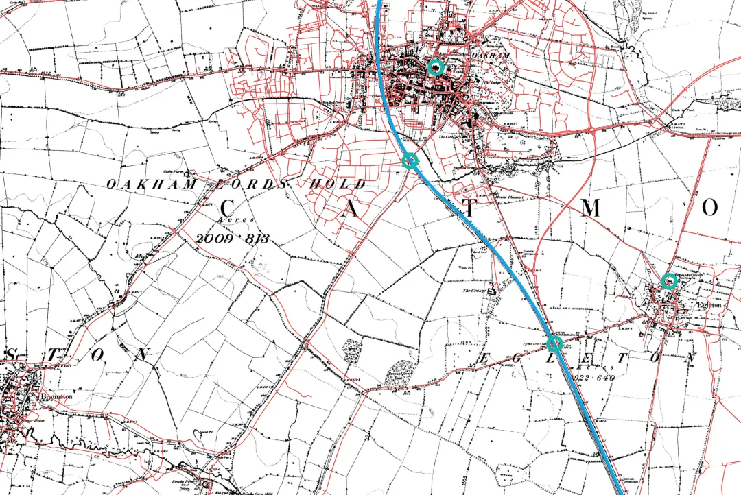
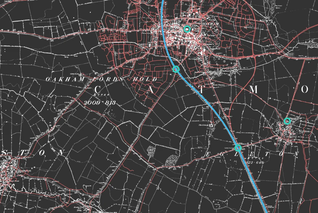
The 1880s Ordnance Survey sheet around Oakham with today's OpenStreetMap roads in red and railway in blue projected onto it through a four-point fit; the railway and old roads line up, the modern bypass crosses open fields. — Today's railway and roads projected through four control points: the old network lines up; the new roads cross 1880s fields.

The blue line is today's railway, landing on the 1880s one along its whole length. Red roads that cross open fields are the modern Oakham bypass and estates — features that cannot be control points because they did not exist.

3. Place each point at full resolution

With the rough fit predicting where each candidate falls, crop the scan around the prediction and place the point by eye:

from PIL import Image

scan = Image.open("data/os_009-NW.jpg")
for name, e, n in [("Barleythorpe Road crossing", 485688.8, 308908.8)]:
    x, y = np.array([e, n, 1]) @ cx, np.array([e, n, 1]) @ cy
    crop = scan.crop((int(x) - 80, int(y) - 80, int(x) + 80, int(y) + 80))
    crop.save("data/candidate.png")
    print(f"{name}: predicted at pixel ({x:.0f}, {y:.0f}); crop saved for inspection")

Barleythorpe Road crossing: predicted at pixel (2730, 483); crop saved for inspection

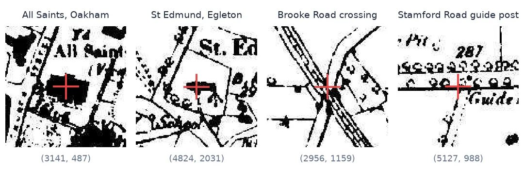
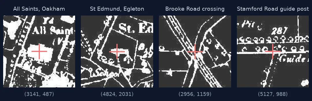
Four close-ups of the scan with a red cross on each chosen control point: the centre of All Saints church in Oakham, the centre of St Edmund's in Egleton, the Brooke Road railway crossing, and the junction at the Stamford Road guide post. — Where each point went: block centres for churches, centre-line meetings for crossings, the junction rather than the symbol for a guide post.

Each pick is a judgement. A church is drawn as a block, so its point goes at the block's centre, which is not where OpenStreetMap's polygon puts it. A road crossing goes where the two centre-lines meet. A guide post marks a junction, and its pixel goes where the lane meets the road, not on the symbol. Writing down what each point is — the id above — is what lets someone check it later.

4. Spread the points over the whole sheet

Points clustered in the town fit the town and let the corners wander. The seven here run from Braunston in the west to the Stamford road in the east and from Oakham to Brooke — and still leave gaps:

px = np.array([p[1] for p in GCPS]); py = np.array([p[2] for p in GCPS])
hull = shapely.MultiPoint(list(zip(px, py))).convex_hull
print(f"control points span {px.min()}–{px.max()} px across and {py.min()}–{py.max()} px down; "
      f"their hull covers {hull.area / (5343 * 3573):.0%} of the sheet")

control points span 1263–5127 px across and 487–3292 px down; their hull covers 35% of the sheet

Their hull covers about a third of the sheet. The north-west and south-east corners have no control point near them, so anything there is extrapolated, and it is where a map georeferenced from these points will be least trustworthy. The fields there offer nothing that is certainly unchanged; the honest course is to say so rather than add a doubtful point.

5. Test every point against the others

The residual of a point in a fit that includes it is flattering: the fit has bent towards it. Leaving each point out and predicting it from the rest — the loop in the quick answer — gives an error you can trust, and it singles out a bad pick: a point that is wrong by 60 pixels stands out from six at 20.

Each point predicted from the other six.

6. Save the points in a format other tools read

lines = ["mapX,mapY,sourceX,sourceY,enable"]
lines += [f"{p[3]},{p[4]},{p[1]},{-p[2]},1" for p in GCPS]          # QGIS stores the line as negative
Path("data/os_009-NW.jpg.points").write_text("\n".join(lines) + "\n")
print(Path("data/os_009-NW.jpg.points").read_text())

mapX,mapY,sourceX,sourceY,enable
486065.6,308906.1,3141,-487,1
487598.5,307540.3,4824,-2031,1
485892.0,308306.8,2956,-1159,1
486838.1,307119.0,3998,-2481,1
487872.3,308486.1,5127,-988,1
484382.4,307839.2,1263,-1675,1
484648.2,306376.1,1547,-3292,1

A .points file next to the image is what the QGIS Georeferencer reads and writes, so points picked in Python can be checked by eye in QGIS, and the reverse. Note that QGIS stores the row as a negative number.

Picking points on sheet Rutland 009-NW

The data used on this page

The Ordnance Survey six-inch sheet Rutland 009-NW, surveyed 1884–1891, from Wikimedia Commons (public domain), and OpenStreetMap for Rutland from Geofabrik's extract of 1 January 2026 (© OpenStreetMap contributors, ODbL).

from pathlib import Path

import geopandas as gpd
import numpy as np
import requests
import shapely

Path("data").mkdir(exist_ok=True)
UA = {"User-Agent": "spatialworkflow.io guide (https://www.spatialworkflow.io)"}
downloads = {
    "data/os_009-NW.jpg": "https://upload.wikimedia.org/wikipedia/commons/a/a0/"
                          "Map_of_Rutland_OS_Map_name_009-NW%2C_Ordnance_Survey%2C_1884-1891.jpg",
    "data/rutland.shp.zip": "https://download.geofabrik.de/europe/united-kingdom/england/rutland-260101-free.shp.zip",
}
for target, url in downloads.items():
    if not Path(target).exists():
        Path(target).write_bytes(requests.get(url, headers=UA, timeout=300).content)
OSM = "/vsizip/data/rutland.shp.zip/"
print({p.name: f"{p.stat().st_size / 1e6:.1f} MB" for p in Path("data").iterdir()})

{'rutland.shp.zip': '2.7 MB', 'os_009-NW.jpg': '2.7 MB'}

Example 1: why automatic snapping did not replace picking by hand

The obvious shortcut is to slide the projected modern roads around each predicted point and keep the offset where they best cover the ink. Tried on the four hand-picked points it should have confirmed:

from PIL import ImageDraw, ImageFilter

gray = Image.open("data/os_009-NW.jpg").convert("L").point(lambda v: 255 - v)
fine = np.asarray(gray.filter(ImageFilter.GaussianBlur(2)), float) / 255
ink = fine - np.asarray(gray.filter(ImageFilter.GaussianBlur(25)), float) / 255   # line-like ink only
lines = list(roads.geometry) + list(gpd.read_file(OSM + "gis_osm_railways_free_1.shp", bbox=bbox).to_crs(27700).geometry)


def snap(e, n, cx, cy, half=150, search=40):
    mask = Image.new("L", (2 * half, 2 * half)); d = ImageDraw.Draw(mask)
    x0, y0 = np.array([e, n, 1]) @ cx - half, np.array([e, n, 1]) @ cy - half
    area = shapely.Point(e, n).buffer(140)
    for g in lines:
        for part in shapely.get_parts(g.intersection(area)):
            if part.geom_type == "LineString":
                c = np.asarray(part.coords)[:, :2]; a = np.c_[c, np.ones(len(c))]
                d.line(list(zip(a @ cx - x0, a @ cy - y0)), fill=255, width=3)
    m = np.asarray(mask, float) / 255
    best = max(((float((ink[int(y0) + dy:int(y0) + dy + 2 * half, int(x0) + dx:int(x0) + dx + 2 * half] * m).sum()), dx, dy)
                for dx in range(-search, search + 1, 2) for dy in range(-search, search + 1, 2)))
    return x0 + half + best[1], y0 + half + best[2]


cx, cy = fit_affine(GCPS[:4])
for p in GCPS[:4]:
    sx, sy = snap(p[3], p[4], cx, cy)
    print(f"{p[0]:24} hand ({p[1]}, {p[2]})  snapped ({sx:.0f}, {sy:.0f})  moved {np.hypot(sx - p[1], sy - p[2]):.0f} px")

oakham_church            hand (3141, 487)  snapped (3153, 487)  moved 12 px
egleton_church           hand (4824, 2031)  snapped (4832, 2014)  moved 18 px
brooke_rd_crossing       hand (2956, 1159)  snapped (2928, 1124)  moved 45 px
egleton_level_crossing   hand (3998, 2481)  snapped (3996, 2497)  moved 16 px

It moved every point, and one by 45 pixels. The reason is the subject itself: roads have been widened, straightened and rebuilt since the 1880s, so the modern line is the wrong template for the old ink, and in a dense town the best-covering offset is wherever the most ink is. Automatic matching works between two scans of the same survey; between a Victorian map and today's network, it needs a person to decide what is the same place.

What Example 1 measured.

Example 2: a point that is wrong

Moving one pick by 60 pixels — a slip to the wrong side of a junction — shows what the leave-one-out test catches:

bad = list(GCPS)
bad[4] = (bad[4][0], bad[4][1] + 60, bad[4][2], bad[4][3], bad[4][4])
for i, p in enumerate(bad):
    cx, cy = fit_affine(bad[:i] + bad[i + 1:])
    e = np.array([p[3], p[4], 1.0])
    print(f"{p[0]:24} {np.hypot(e @ cx - p[1], e @ cy - p[2]):5.1f} px")

oakham_church             29.1 px
egleton_church            39.1 px
brooke_rd_crossing         5.0 px
egleton_level_crossing    13.0 px
stamford_rd_guide_post    42.7 px
braunston_rd_bridleway    17.4 px
brooke_guide_post         15.5 px

The bad point now has the largest error, 42.7 pixels — but only just. Egleton church, its nearest neighbour on the east side, jumps from 9.3 to 39.1, because it is predicted by a fit that includes the bad point and has nothing else nearby to hold it. With seven points one bad pick spreads; compare the errors with the clean run, not just with each other, and when one point and its neighbour both jump, check the one that moved.

A control point is a claim

A control point is a claim that two things are the same place: this pixel on the scan, and this coordinate today. Everything after — the transformation, the warp, the accuracy you quote — rests on those claims, so the quality of a georeferenced map is set when the points are picked.

The features that make good claims share three properties. They are unchanged: a medieval church or a railway built in the 1840s is where it was; a hedge or a field corner may not be. They are unambiguous: a level crossing is one point, while a bend in a lane is a judgement. And they are identifiable in both datasets with the same convention: a church block's centre on the scan is not the same as the centroid of OpenStreetMap's building outline, and the few metres between them are part of the error.

The rough-fit-then-refine workflow exists because the scan is large and the features are small. Projecting today's network through a fit from four easy points turns a search over 19 million pixels into a glance at a 160-pixel crop, and the overlay itself shows at once which modern features are new — the bypass, the estates — and so cannot be used.

Leave-one-out testing is what makes the error honest. With seven points and an affine fit of six parameters, the fit cannot match every point exactly, and the residuals it reports are biased low because each point helped shape the fit. Predicting each point from the others answers the question that matters: how far off will a place be that was not used as a control point? Here, 8 to 22 metres.

Point counts, spread and map symbols

Use at least six points for an affine fit, more for polynomial or spline transformations, so leave-one-out has something to test.
Spread matters more than number. Ten points in the town fit the town; the corners need their own.
Map symbols are not positions. A church, a guide post or a milestone is drawn beside or around the point it marks.
Sheet edges are not control points on these scans: the paper margins were trimmed.
Record what each point is. An id like egleton_level_crossing makes a later check possible; a bare pair of numbers does not.
QGIS .points files store the row as negative, and GDAL's -gcp options take pixel, line, easting, northing in that order.
Old maps have their own grid. The half-degree rotation found here is the difference between the Ordnance Survey's county projection and the National Grid, not a scanning error.

Internal links

Ground control points explained — how many, where, and how good
How to georeference a scanned map with GDAL — using these points
How to compare georeferencing transformations — affine, polynomial and spline from the same points
How to find and download scanned historical maps — where the sheet came from
GCP residuals are low but the map is still wrong — when the numbers flatter

FAQ

How many ground control points do I need?

Three is the minimum for an affine transformation, but use at least six so you can test each one against the others. More points help only if they add coverage of the sheet or replace doubtful ones.

What makes a good ground control point?

A feature that has not moved since the map was made, that is a single unambiguous point, and that you can locate the same way on both maps: church centres, railway crossings, old bridges and road junctions that have not been rebuilt.

Can I pick control points automatically?

Between two scans of the same survey, often yes. Between an old map and today's data, automatic matching against modern roads moved hand-picked points by up to 45 pixels on the Oakham sheet, because the roads themselves have changed. Use automation to predict where to look, and a person to decide.

Why are my residuals small but the map still looks wrong?

Residuals measured on the points that built the fit are optimistic. Leave each point out and predict it from the others; that error is what you should quote.

Where should I place a point on a church?

Somewhere you can define the same way in both datasets. The middle of the building block is reasonable on a six-inch map; make sure the modern coordinate is the middle of the same building, not a centroid of a larger churchyard polygon.