
How to Georeference a Scanned Map with GDAL in Python
On this page
Problem statement
You have a scanned map and a set of ground control points — pixel positions paired with real coordinates — and you want a GeoTIFF that sits in the right place in QGIS, a web map or a raster analysis. GDAL does this in two steps, and both have defaults that quietly produce a worse file than you wanted: a 58 MB output from a 2.7 MB scan, three identical colour bands, and a "nodata" value that makes the map's own ink transparent.
This page georeferences the Ordnance Survey six-inch sheet of Oakham, surveyed 1884–1891, onto British National Grid with the seven control points picked in the control-point guide, and measures what each choice does to the result.
Quick answer
Attach the control points in a VRT, then warp to the target CRS with an explicit resolution, an alpha band and compression:
from osgeo import gdal
gdal.UseExceptions()

gcps = [gdal.GCP(e, n, 0, px, py, name) for name, px, py, e, n in GCPS]
gdal.Translate("data/os_gcps.vrt", "data/os_009-NW.jpg", format="VRT",
               GCPs=gcps, outputSRS="EPSG:27700", bandList=[1])          # one grey band
gdal.Warp("data/oakham_1880s.tif", "data/os_gcps.vrt", dstSRS="EPSG:27700",
          polynomialOrder=1, xRes=1, yRes=1, resampleAlg="cubic", dstAlpha=True,
          creationOptions=["COMPRESS=DEFLATE", "TILED=YES", "PREDICTOR=2"])

info = gdal.Info("data/oakham_1880s.tif", format="json")
print(info["size"], info["bands"][-1]["colorInterpretation"], info["coordinateSystem"]["wkt"].split('"')[1])
print([round(v) for v in info["cornerCoordinates"]["upperLeft"]], round(Path("data/oakham_1880s.tif").stat().st_size / 1e6, 1), "MB")
[4843, 3258] Alpha OSGB36 / British National Grid
[483228, 309370] 5.2 MB
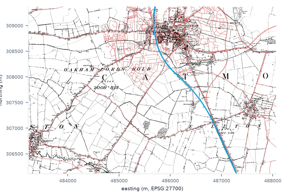
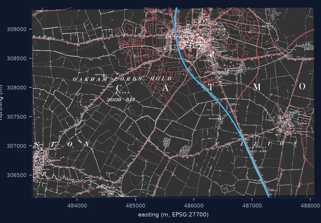
A 1 m grid in British National Grid, one grey band plus alpha, about 5 MB. The sheet now lines up with today's data:
Control points in a VRT, chosen resolution, alpha not zero
1. Attach the control points in a VRT
gdal.Translate with GCPs= writes the points into a small VRT that refers to the scan; nothing is resampled yet. The scan still has its pixel grid, but it now carries the information needed to compute a transformation:
gdal.Translate("data/os_rgb_gcps.vrt", "data/os_009-NW.jpg", format="VRT", GCPs=gcps, outputSRS="EPSG:27700")
vrt = gdal.Open("data/os_rgb_gcps.vrt")
print(vrt.GetGCPCount(), "GCPs,", vrt.RasterCount, "bands,", gdal.GetDataTypeName(vrt.GetRasterBand(1).DataType),
      "| geotransform until warped:", vrt.GetGeoTransform())
7 GCPs, 3 bands, Byte | geotransform until warped: (0.0, 1.0, 0.0, 0.0, 0.0, 1.0)
gdal.GCP takes the world coordinate first and the pixel second — GCP(x, y, z, pixel, line) — which is the reverse of the order in which you picked them. Keeping the points as named tuples and building the GCP objects in one line is the simplest way not to swap them.
2. Drop bands that carry nothing
The scan is a JPEG with three colour channels, but the map is black ink on white paper:
a = vrt.ReadAsArray()
print("bands identical:", bool((a[0] == a[1]).all() and (a[1] == a[2]).all()))
bands identical: True
All three bands are the same, so keeping them triples the size of everything downstream. bandList=[1] in the translate step keeps one.
3. Choose the resolution instead of accepting it
Without xRes/yRes, gdal.Warp picks a resolution that roughly preserves the number of pixels:
for label, kw in (("default", {}), ("1 m", dict(xRes=1, yRes=1))):
    ds = gdal.Warp("", "data/os_gcps.vrt", format="MEM", dstSRS="EPSG:27700", polynomialOrder=1, **kw)
    gt = ds.GetGeoTransform()
    print(f"{label:8} {ds.RasterXSize} x {ds.RasterYSize} px at {gt[1]:.3f} m")
default 5375 x 3615 px at 0.901 m
1 m 4843 x 3258 px at 1.000 m
The default is 0.901 m — an accident of this scan's dots per inch. A round 1 m is close to the scan's own detail, aligns cleanly with other British National Grid rasters and makes every later calculation simpler. Choose it.
4. Mark outside the sheet with alpha, not with nodata 0
A rotated sheet on a north-up grid leaves wedges at the corners that the map does not cover. GDAL fills them with 0 unless told otherwise, and the usual next step — declaring 0 as nodata — has a catch on a map:
scan = gdal.Open("data/os_gcps.vrt").ReadAsArray()
print(f"pixels of the scan that are already 0: {(scan == 0).mean():.1%}")
pixels of the scan that are already 0: 3.1%
Three per cent of the sheet is pure black ink. Declare 0 as nodata and every one of those pixels becomes transparent — the solid church blocks, the castle, the heaviest lettering:
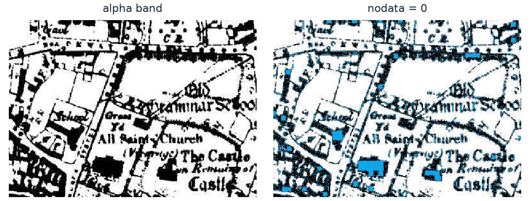
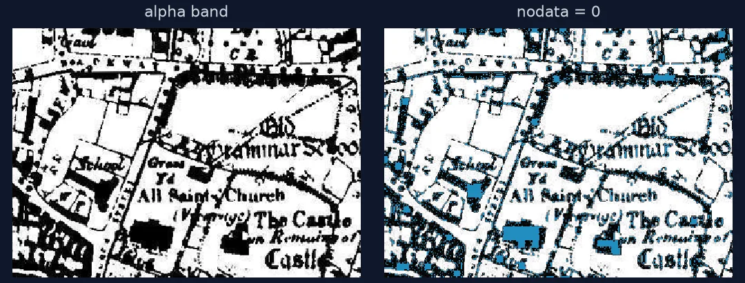
dstAlpha=True adds a fourth band that is 0 only where the warp had no source pixel, which keeps the ink and still lets the wedges show through. If you must use a nodata value, pick one the scan never uses.
5. Compress, and measure what you saved
import os

variants = {
    "RGB, uncompressed": dict(),
    "grey + alpha, DEFLATE": dict(dstAlpha=True, creationOptions=["COMPRESS=DEFLATE", "TILED=YES", "PREDICTOR=2"]),
}
for label, kw in variants.items():
    src = "data/os_rgb_gcps.vrt" if label.startswith("RGB") else "data/os_gcps.vrt"
    gdal.Warp("data/variant.tif", src, dstSRS="EPSG:27700", polynomialOrder=1, xRes=1, yRes=1,
              resampleAlg="cubic", **kw)
    print(f"{label:24} {os.path.getsize('data/variant.tif') / 1e6:5.1f} MB")
RGB, uncompressed 47.4 MB
grey + alpha, DEFLATE 5.2 MB
Black-and-white linework compresses extremely well losslessly; the right options turn a file seventeen times the size of the scan into one about twice its size, with nothing lost.
6. Check the result against data you trust
The overlay at the top of the page is the check that matters: today's railway sits on the Victorian one along the whole sheet, and the old lanes run under their modern successors. For a number, use the leave-one-out error from the control points — 8 to 22 m on this sheet — and quote that, not the residuals of the fit.
The same steps from the command line
The data used on this page
The Ordnance Survey six-inch sheet Rutland 009-NW (1884–1891) from Wikimedia Commons (public domain), and the seven control points picked against OpenStreetMap (Geofabrik, 1 January 2026; © OpenStreetMap contributors, ODbL) in the control-point guide.
import sys
from pathlib import Path

import requests

Path("data").mkdir(exist_ok=True)
UA = {"User-Agent": "spatialworkflow.io guide (https://www.spatialworkflow.io)"}
scan = Path("data/os_009-NW.jpg")
if not scan.exists():
    scan.write_bytes(requests.get("https://upload.wikimedia.org/wikipedia/commons/a/a0/"
                                  "Map_of_Rutland_OS_Map_name_009-NW%2C_Ordnance_Survey%2C_1884-1891.jpg",
                                  headers=UA, timeout=300).content)
GCPS = [  # (id, pixel, line, easting, northing)
    ("oakham_church",          3141,  487, 486065.6, 308906.1),
    ("egleton_church",         4824, 2031, 487598.5, 307540.3),
    ("brooke_rd_crossing",     2956, 1159, 485892.0, 308306.8),
    ("egleton_level_crossing", 3998, 2481, 486838.1, 307119.0),
    ("stamford_rd_guide_post", 5127,  988, 487872.3, 308486.1),
    ("braunston_rd_bridleway", 1263, 1675, 484382.4, 307839.2),
    ("brooke_guide_post",      1547, 3292, 484648.2, 306376.1),
]
print(scan.stat().st_size, "bytes;", len(GCPS), "control points")
2653911 bytes; 7 control points
Example 1: the same thing with the command-line tools
gdal_translate and gdalwarp take the same options, which is useful when the job runs in a shell script:
gcp_args = " ".join(f"-gcp {px} {py} {e} {n}" for _, px, py, e, n in GCPS)
!gdal_translate -q -of VRT -b 1 -a_srs EPSG:27700 {gcp_args} data/os_009-NW.jpg data/cli.vrt
!gdalwarp -q -overwrite -t_srs EPSG:27700 -order 1 -tr 1 1 -r cubic -dstalpha -co COMPRESS=DEFLATE -co TILED=YES -co PREDICTOR=2 data/cli.vrt data/cli.tif
!gdalinfo data/cli.tif | grep -E "^Size|^Origin|^Band"
Size is 4843, 3258
Origin = (483228.135366102680564,309370.059889321273658)
Band 1 Block=256x256 Type=Byte, ColorInterp=Red
Band 2 Block=256x256 Type=Byte, ColorInterp=Alpha
On the command line the order is pixel, line, easting, northing — the opposite of the Python gdal.GCP constructor, and the source of many maps in the wrong place.
Example 2: write the transformation into the file instead of resampling
If the map only needs to be displayed, you can skip the warp and store the fitted affine transformation as a geotransform:
import numpy as np

P = np.array([[g[1], g[2]] for g in GCPS], float)
W = np.c_[np.array([[g[3], g[4]] for g in GCPS]), np.ones(len(GCPS))]
inv_x = np.linalg.lstsq(np.c_[P, np.ones(len(P))], W[:, 0], rcond=None)[0]       # pixel -> easting
inv_y = np.linalg.lstsq(np.c_[P, np.ones(len(P))], W[:, 1], rcond=None)[0]       # pixel -> northing
gt = (inv_x[2], inv_x[0], inv_x[1], inv_y[2], inv_y[0], inv_y[1])
ds = gdal.Translate("data/oakham_geotransform.tif", "data/os_009-NW.jpg", bandList=[1], outputSRS="EPSG:27700",
                    creationOptions=["COMPRESS=DEFLATE", "TILED=YES"])
ds.SetGeoTransform(gt)
ds = None
print("rotation terms:", round(gt[2], 4), round(gt[4], 4), "| pixel size:", round(gt[1], 4), round(gt[5], 4))
rotation terms: 0.0054 0.0076 | pixel size: 0.9028 -0.9004
The non-zero rotation terms are the half-degree turn between the old county grid and the National Grid. QGIS and GDAL honour them; many web tools and some libraries do not, and will draw the sheet north-up in the wrong place. A rotated geotransform is a fine archival format and a poor exchange format — warp before you share.
Where the pixels go, and how they are warped
Georeferencing with GDAL separates two questions: where is each pixel, and what should the new grid look like. The control points answer the first, through a transformation fitted to them. The warp answers the second: it builds an empty grid in the target CRS, at the resolution you ask for, and fills each cell by asking the transformation where that cell came from on the scan.
That inverse direction explains the outputs. Cells whose source falls outside the scan have no value, which is why the corners need an alpha band. Cells between scan pixels need interpolating, which is what resampleAlg chooses — cubic keeps thin lines crisper than nearest neighbour without the blur of bilinear. And the output grid's resolution is a free choice, not a property of the scan, which is why the default of 0.901 m is worth overriding.
The format choices follow from what the image is. A scan of a printed map is greyscale linework, so one band and lossless compression fit it; a hand-coloured map would keep its colour bands. The nodata trap is specific to maps: a satellite image rarely has exactly 0 in its data, but a black-and-white scan has a great deal of it, and the convention that 0 means "no data" erases precisely the darkest, most important features.
GCP argument order, CRS declarations and nodata
gdal.GCP(x, y, z, pixel, line)is world-first;-gcp pixel line x yon the command line is pixel-first.- Declare the CRS of the control points with
outputSRS/-a_srs, or the warp has nothing to transform from. - JPEG scans are often three identical bands; check before keeping all three.
- Never use 0 as nodata on a black-and-white scan. Use an alpha band or a value the scan does not contain.
- Resolution is your choice. Pick a round number in the target CRS's units.
- Cubic resampling keeps linework crisper than bilinear; nearest neighbour keeps exact grey values if you plan to threshold.
- A rotated geotransform displays correctly in GDAL and QGIS but not everywhere; warp before sharing.
Internal links
- Georeferencing explained — the idea behind every step here
- How to pick ground control points for a scanned map — where the seven points came from
- How to compare georeferencing transformations — affine, polynomial and spline on this sheet
- Georeferenced map has a black border or hides other layers — the nodata problem in detail
- How to overlay a georeferenced old map on a web map — the next step for sharing it
FAQ
How do I georeference an image with GDAL in Python?
Add the control points with gdal.Translate(..., GCPs=[gdal.GCP(x, y, 0, pixel, line)], outputSRS=...), then gdal.Warp to the target CRS with a transformation (polynomialOrder=1 for affine, tps=True for a thin-plate spline), a resolution and an alpha band.
Why is my georeferenced GeoTIFF so large?
Three identical bands, no compression and a resolution finer than you need. One band, DEFLATE with a predictor and a round resolution took the Oakham sheet from 47 MB at 1 m in RGB to about 5 MB.
Why have parts of my map become transparent?
0 is being treated as nodata, and your map's black ink is 0. Use an alpha band (dstAlpha=True) instead.
Should I warp or just set a geotransform?
A geotransform with rotation terms avoids resampling and is fine for GDAL and QGIS. For anything else — web tiles, other software, analysis with other rasters — warp to a north-up grid.
Which resampling method should I use for a scanned map?
Cubic for viewing; nearest neighbour if you will later threshold the image into ink and paper, because it keeps the original grey values.