How to Fit Ground-Motion Attenuation to ShakeMap Stations in Python

Problem statement

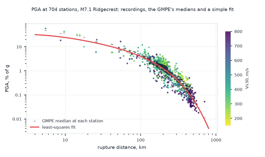
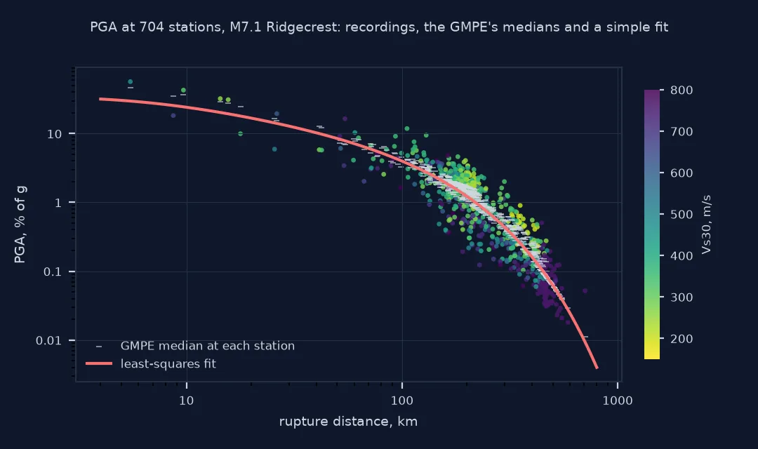
Shaking weakens with distance from an earthquake, quickly at first and then more slowly, and how it weakens is the core of every seismic hazard model and every ShakeMap. Those models are ground-motion prediction equations (GMPEs), fitted to thousands of recordings from many earthquakes. One large, well-recorded earthquake is enough to see the shape for yourself: fit a simple attenuation curve to its station data, compare the recordings with the model ShakeMap used, and split the misfit into a part common to the whole event and a part that varies from site to site.

This page fits an attenuation curve to the peak ground accelerations recorded at 704 stations during the 2019 M7.1 Ridgecrest earthquake, compares the recordings with the GMPE predictions ShakeMap lists for each station, and tests whether soft sites recorded stronger shaking.

Quick answer

Fit ln PGA = c0 + c1 ln √(R² + h²) + c2 R to the stations by least squares:

h = 6.0
Rh = np.sqrt(A.rrup ** 2 + h ** 2)
X = np.column_stack([np.ones(len(A)), np.log(Rh), Rh])
c, *_ = np.linalg.lstsq(X, np.log(A.pga), rcond=None)
resid = np.log(A.pga) - X @ c
print(f"ln PGA = {c[0]:.2f} {c[1]:+.3f} ln(sqrt(R^2 + {h:.0f}^2)) {c[2]:+.5f} R   (PGA in % of g, R in km)")
print(f"{len(A)} stations; residual standard deviation {resid.std():.2f} (a factor of {np.exp(resid.std()):.2f})")

ln PGA = 4.49 -0.492 ln(sqrt(R^2 + 6^2)) -0.00840 R   (PGA in % of g, R in km)
704 stations; residual standard deviation 0.61 (a factor of 1.84)

The fitted curve has a geometric spreading coefficient of -0.492 and an anelastic term of -0.0084 per km. Around it the recordings scatter with a standard deviation of 0.61 in natural-log units: one standard deviation is a factor of 1.84 either way, typical for ground motion from one earthquake at many sites.

Look at the data, compare the model, consider site effects

1. Look at the data first

Bin the recordings by distance and take medians; PGA spans more than three orders of magnitude:

bins = pd.cut(A.rrup, [0, 10, 20, 50, 100, 200, 400, 900])
print(A.groupby(bins, observed=True).pga.agg(stations="size", median="median", lowest="min", highest="max").round(2).to_string())

            stations  median  lowest  highest
rrup                                         
(0, 10]            3   42.87   18.31    56.91
(10, 20]           3   31.12    9.96    32.19
(20, 50]           4    5.88    5.76    19.50
(50, 100]         24    4.37    1.63    16.46
(100, 200]       236    2.01    0.19    11.85
(200, 400]       300    0.64    0.06     3.40
(400, 900]       134    0.09    0.02     0.55

The median PGA falls from 42.9% of g within 10 km to 2.0% at 100–200 km and 0.09% beyond 400 km. Near the rupture there are only ten stations within 50 km, and their values vary by a factor of three in each band; most of the information about the shape of the curve comes from the hundreds of stations beyond 100 km.

2. Compare with the model ShakeMap used

Each station in the list carries the GMPE's median prediction for its distance and site. The mean log residual is the event term, how much stronger or weaker this earthquake was than the model's average:

A["ln_res"] = np.log(A.pga / A.pred)
print(f"event term (mean ln residual): {A.ln_res.mean():+.3f}, a factor of {np.exp(A.ln_res.mean()):.2f}")
print(f"ShakeMap's own bias estimate for PGA: {A.ln_bias.iloc[0]:+.3f}")
print(f"within-event standard deviation: {A.ln_res.std():.3f}; model's phi {A.ln_phi.median():.3f}, tau {A.ln_tau.median():.3f}")
print(A.groupby(bins, observed=True).ln_res.agg(["size", "mean"]).round(2).to_string())

event term (mean ln residual): -0.109, a factor of 0.90
ShakeMap's own bias estimate for PGA: -0.035
within-event standard deviation: 0.550; model's phi 0.526, tau 0.321
            size  mean
rrup                  
(0, 10]        3 -0.10
(10, 20]       3 -0.23
(20, 50]       4 -0.58
(50, 100]     24 -0.18
(100, 200]   236 -0.05
(200, 400]   300 -0.16
(400, 900]   134 -0.06

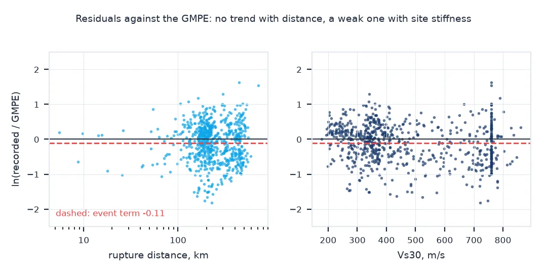
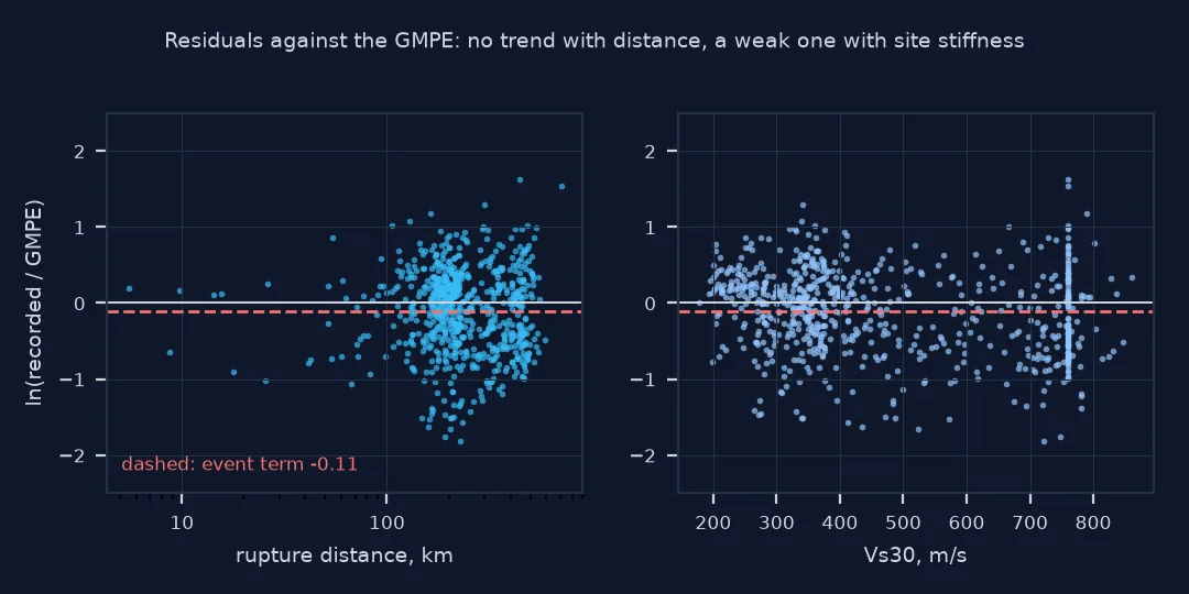
On average the recordings are 10% below the GMPE's medians, a mean log residual of -0.109. ShakeMap's own bias estimate is smaller, -0.035; it is not a simple mean of these residuals, but both say this earthquake's PGA was slightly below the model's average for its magnitude. The scatter within the event, 0.550, is close to the model's phi, 0.526, and smaller than the simple fit's 0.61. By distance, the residuals are within about ±0.25 except for the four stations at 20–50 km, which recorded 44% less than predicted.

3. Site effects

Soft soils amplify shaking. The GMPE accounts for that through Vs30, so residuals from the simple distance-only fit should depend on Vs30 and residuals from the GMPE should not:

soft, rock = A.vs30 < 300, A.vs30 >= 600
for name, r in (("distance-only fit", resid), ("ShakeMap GMPE", A.ln_res)):
    print(f"{name:>17}: soft sites (Vs30 < 300, n={soft.sum()}) {r[soft].mean():+.2f}; rock (Vs30 >= 600, n={rock.sum()}) {r[rock].mean():+.2f}; "
          f"correlation with ln Vs30 {np.corrcoef(np.log(A.vs30), r)[0, 1]:+.2f}")

distance-only fit: soft sites (Vs30 < 300, n=141) +0.36; rock (Vs30 >= 600, n=206) -0.30; correlation with ln Vs30 -0.43
    ShakeMap GMPE: soft sites (Vs30 < 300, n=141) +0.02; rock (Vs30 >= 600, n=206) -0.21; correlation with ln Vs30 -0.19

Against the distance-only fit, the 141 soft-soil stations recorded 43% more than the curve (+0.36) and the 206 rock stations 26% less (-0.30): a clear site effect, with a correlation of -0.43 between residual and ln Vs30. The GMPE removes most of it for soft sites, whose mean residual is +0.02, but rock sites are still 19% below its predictions and a weaker correlation, -0.19, remains.

Predicted shaking at round distances

The data used on this page

The station list of the preferred ShakeMap for the M7.1 Ridgecrest earthquake of 6 July 2019 (USGS event ci38457511), from the event's entry in the USGS FDSN event service. The setup keeps seismic stations with a PGA and no flagged amplitude, and takes the GMPE's PGA prediction and uncertainties from each station's predictions.

import json
from pathlib import Path

import numpy as np
import pandas as pd
import requests

Path("data").mkdir(exist_ok=True)
EV = "ci38457511"
p = Path(f"data/{EV}.json")
if not p.exists():
    r = requests.get("https://earthquake.usgs.gov/fdsnws/event/1/query", params={"eventid": EV, "format": "geojson"}, timeout=120)
    r.raise_for_status()
    p.write_text(r.text)
pr = json.loads(p.read_text())["properties"]["products"]["shakemap"][0]
st = Path(f"data/{EV}_shakemap_{pr['source']}_stationlist.json")
if not st.exists():
    r = requests.get(pr["contents"]["download/stationlist.json"]["url"], timeout=600)
    r.raise_for_status()
    st.write_bytes(r.content)
rows = []
for f in json.loads(st.read_text())["features"]:
    q = f["properties"]
    if q["station_type"] != "seismic" or q.get("pga") in (None, "null"):
        continue
    if any(a.get("flag", "0") not in ("0", "") for ch in q["channels"] for a in ch["amplitudes"]):
        continue
    pga = next(x for x in q["predictions"] if x["name"] == "pga")
    rows.append({"code": f"{q['network']}.{q['code']}", "pga": float(q["pga"]), "rrup": q["distances"]["rrup"], "vs30": q["vs30"],
                 "pred": pga["value"], "ln_bias": pga["ln_bias"], "ln_phi": pga["ln_phi"], "ln_tau": pga["ln_tau"]})
A = pd.DataFrame(rows)
A = A[A.pga > 0].reset_index(drop=True)
print(f"stations kept: {len(A)}; distances {A.rrup.min():.1f} to {A.rrup.max():.0f} km; PGA {A.pga.min():.3f} to {A.pga.max():.1f} % of g")

stations kept: 704; distances 5.5 to 706 km; PGA 0.018 to 56.9 % of g

704 stations remain after dropping DYFI entries, stations without a PGA and any station with a flagged amplitude. They run from 5.5 to 706 km from the rupture and their PGA from 0.018 to 56.9% of g, a range of more than three thousand.

Example 1: predicted shaking at round distances

Evaluate the fitted curve and the GMPE's medians near a few distances:

for r in (5, 10, 25, 50, 100, 200):
    fit = np.exp(c[0] + c[1] * np.log(np.sqrt(r ** 2 + h ** 2)) + c[2] * np.sqrt(r ** 2 + h ** 2))
    near = A[(A.rrup > r / 1.3) & (A.rrup < r * 1.3)]
    gm = f"GMPE median at {len(near)} stations {near.pred.median():.2f}, recorded {near.pga.median():.2f}" if len(near) else "no stations nearby"
    print(f"R = {r:>3} km: fit {fit:.2f} % of g; {gm}")

R =   5 km: fit 30.39 % of g; GMPE median at 1 stations 46.94, recorded 56.91
R =  10 km: fit 24.15 % of g; GMPE median at 2 stations 35.64, recorded 30.59
R =  25 km: fit 14.54 % of g; GMPE median at 2 stations 15.84, recorded 12.72
R =  50 km: fit 8.49 % of g; GMPE median at 9 stations 8.01, recorded 6.10
R = 100 km: fit 3.98 % of g; GMPE median at 35 stations 3.76, recorded 4.09
R = 200 km: fit 1.22 % of g; GMPE median at 343 stations 1.46, recorded 1.49

Close to the fault the simple curve is too low: 30% of g at 5 km against 57% recorded at the one station there. A single h cannot capture saturation near a 50 km rupture. From 25 km outwards the fit, the GMPE and the recordings agree within about 40%; at 100 km within 10% and at 200 km within about 20%.

Geometric spreading and anelastic loss

Two effects make shaking decay. Geometric spreading spreads the energy of the waves over a growing wavefront, so amplitude falls roughly in proportion to 1/R for body waves, which is the logarithmic term; anelastic attenuation turns a little energy into heat for every kilometre travelled, which is the linear term. The fictitious depth h stops the prediction from going to infinity at zero distance and stands in for the fact that a large rupture is not a point: near the fault, shaking saturates.

Real GMPEs add terms for magnitude, fault type, depth, site conditions through Vs30, basin depth and the hanging wall, and they are fitted to many earthquakes so that the event term averages out. Their uncertainty is split into tau, the variation between earthquakes, and phi, the variation between sites in one earthquake. One earthquake's recordings constrain the event term well, which is exactly what ShakeMap estimates and removes as its bias correction, and leave phi as the irreducible scatter from site to site.

Distance metrics, logarithms and spectral periods

• Distance metric: rupture distance (rrup) is to the nearest point of the fault; for a 50 km rupture, epicentral distance would put near-fault stations far too far away.
• Fitting in logarithms: ground motions are log-normally distributed; fitting PGA itself would let a few large values dominate.
• Clipped or flagged records: drop amplitudes ShakeMap flagged; a clipped near-fault record understates the shaking.
• Spectral periods: long-period motion decays more slowly than PGA; fit each intensity measure separately.

Internal links

• How to compare ShakeMap station data with the grid in Python — the station list
• Ground motion explained — PGA, PGV and intensity
• Seismic hazard explained — where GMPEs are used

FAQ

What is a ground-motion prediction equation?

An empirical model that gives the median and standard deviation of a ground-motion measure, such as PGA, as a function of magnitude, distance, site conditions and other variables.

How do I fit an attenuation curve in Python?

Take the natural logarithm of the recorded ground motion and fit it by least squares against ln of distance (with a fictitious depth) and distance, using numpy.linalg.lstsq.

What is an event term?

The mean residual of all recordings of one earthquake against a GMPE: how much stronger or weaker that earthquake was than the model's average for its magnitude.

Why do soft soils shake more?

Seismic waves slow down and amplify as they enter low-velocity material near the surface; Vs30, the average shear-wave velocity in the top 30 m, is the usual proxy.