
How to Calculate Road Death Rates per Vehicle Mile in Python
On this page
Problem statement
Road deaths per resident tell you how many people a state loses; they do not tell you how dangerous its roads are, because people in some states drive two or three times as far as in others. The standard exposure-based rate divides deaths by vehicle miles travelled (VMT), usually per 100 million miles. The Federal Highway Administration publishes VMT for each state, split into rural and urban roads, in its Highway Statistics table VM-2, an Excel sheet with multi-row headers. Joined to FARS, it gives a second ranking of states and a direct comparison of rural and urban roads.
This page reads VM-2 for 2023, joins it to FARS 2023 deaths, computes deaths per 100 million VMT by state, compares the ranking with deaths per resident, and splits deaths and travel between rural and urban roads.
Quick answer
Read the VM-2 sheet without headers, keep the rows with a state code, and divide FARS deaths by total VMT:
deaths = A.groupby("STATE").FATALS.sum()
T = VM2.join(deaths.rename("deaths")).join(POP.set_index("STATE").POPESTIMATE2023.rename("residents")).astype({"deaths": int})
T["per_100m_vmt"] = T.deaths / (T.vmt_total * 1e6) * 1e8               # VM-2 is in millions of miles
T["per_100k_res"] = T.deaths / T.residents * 1e5
print(f"US: {T.deaths.sum() / T.vmt_total.sum() / 1e6 * 1e8:.2f} deaths per 100 million VMT; {T.vmt_total.sum() / 1e6:.2f} trillion miles")
print(T.sort_values("per_100m_vmt", ascending=False)[["state", "deaths", "per_100m_vmt", "per_100k_res"]].head(4).round(2).to_string(index=False))
US: 1.26 deaths per 100 million VMT; 3.25 trillion miles
state deaths per_100m_vmt per_100k_res
Mississippi 733 1.79 24.93
Arizona 1308 1.74 17.60
South Carolina 1047 1.72 19.48
Kentucky 814 1.66 17.98
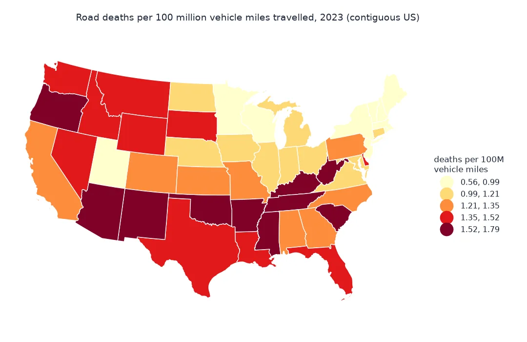
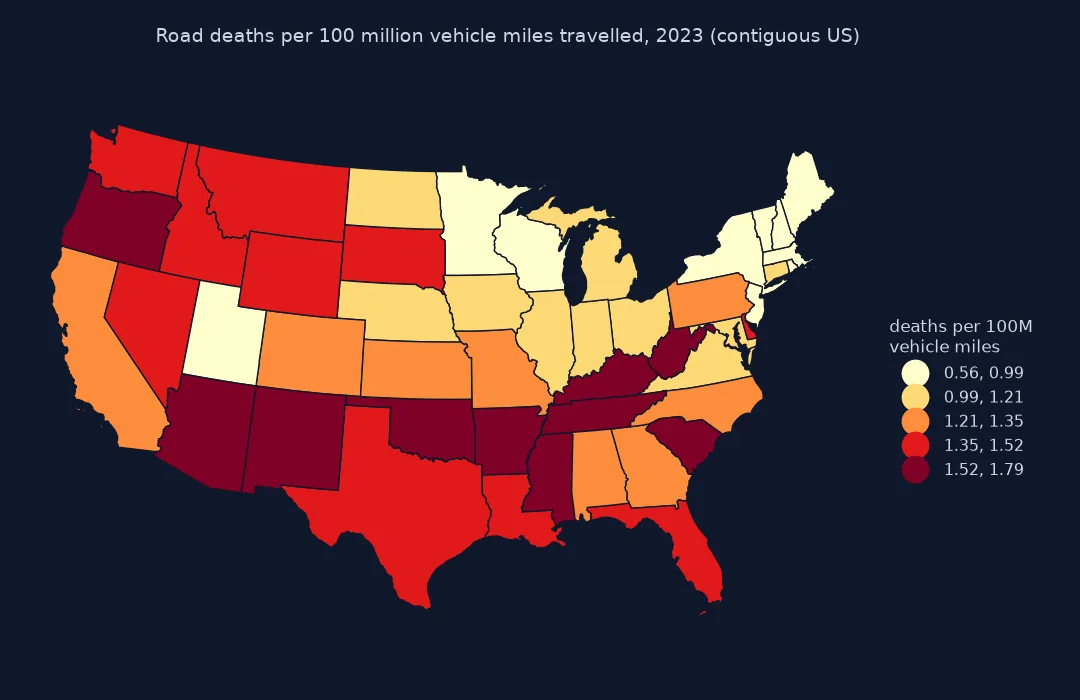
Americans drove 3.25 trillion vehicle miles in 2023, and 41,025 died, 1.26 deaths per 100 million miles. Mississippi tops both rankings, at 1.79 per 100 million miles; Arizona, South Carolina and Kentucky follow per mile.
Parse the VM-2 sheet, compare rankings, split rural and urban
1. Parse the VM-2 sheet
The sheet has six header rows and footnote rows, with rural columns, urban columns and a grand total, followed by the state FIPS code. Check the parsed totals against the sheet:
print(f"rows parsed: {len(VM2)}; columns used: rural total, urban total, total")
print(f"rural + urban = total for every state: {(VM2.vmt_rural + VM2.vmt_urban - VM2.vmt_total).abs().max():.3f} million miles largest gap")
print(VM2.sort_values("vmt_total", ascending=False).head(3)[["state", "vmt_total"]].round(0).to_string(index=False))
rows parsed: 51; columns used: rural total, urban total, total
rural + urban = total for every state: 0.000 million miles largest gap
state vmt_total
California 316612.0
Texas 300338.0
Florida 239188.0
Rural and urban travel add up to the total in every row, and California, Texas and Florida drive the most, 317, 300 and 239 billion miles.
2. Compare the two rankings
T["rank_vmt"] = T.per_100m_vmt.rank(ascending=False).astype(int)
T["rank_res"] = T.per_100k_res.rank(ascending=False).astype(int)
T["miles_per_resident"] = T.vmt_total * 1e6 / T.residents
print(f"rank correlation of the two rates: {T.per_100m_vmt.corr(T.per_100k_res, method='spearman'):.2f}")
moved = (T.rank_vmt - T.rank_res)
print(T.loc[moved.abs().sort_values(ascending=False).index[:4], ["state", "per_100k_res", "per_100m_vmt", "rank_res", "rank_vmt", "miles_per_resident"]].round(2).to_string(index=False))
rank correlation of the two rates: 0.85
state per_100k_res per_100m_vmt rank_res rank_vmt miles_per_resident
District of Columbia 6.48 1.26 47 26 5126.48
Indiana 13.17 1.06 23 38 12417.18
Alabama 19.07 1.35 6 21 14150.74
Oregon 13.87 1.59 21 6 8696.62
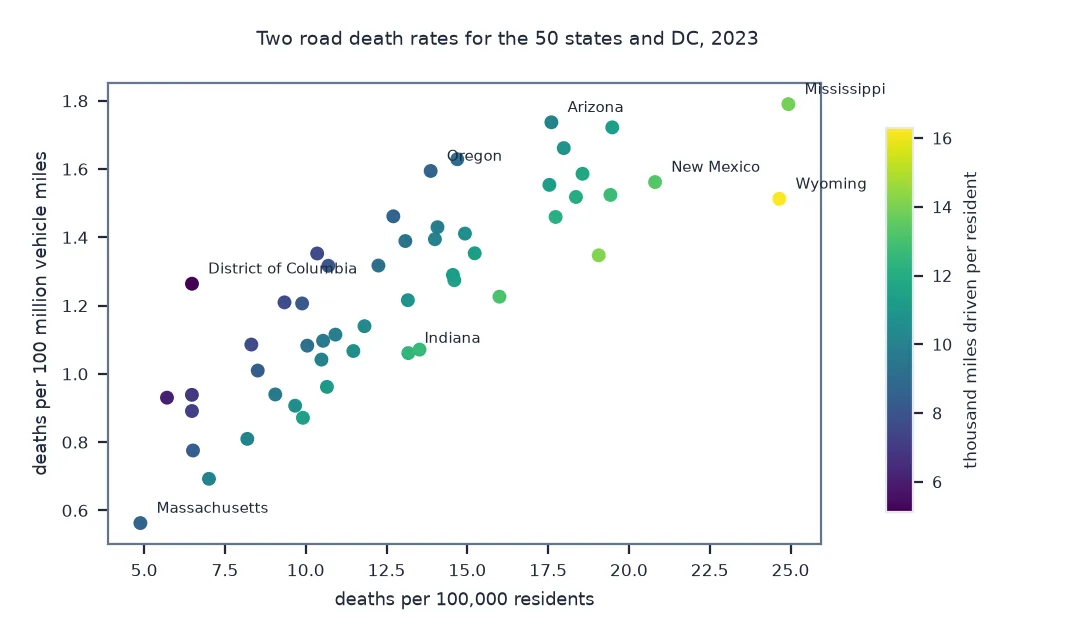
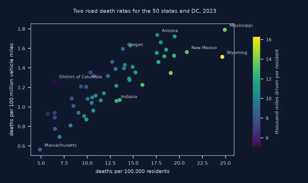
The two rates agree broadly, a rank correlation of 0.85, with large moves for a few. Washington DC goes from 47th per resident to 26th per mile, because its residents drive 5,126 miles a year each; Oregon rises from 21st to 6th per mile, and Alabama and Indiana fall when their long annual mileage is taken into account.
3. Split rural and urban roads
FARS classifies each crash as rural or urban, as VM-2 does for travel. Divide each group's deaths by its travel:
dr = A[A.RUR_URBNAME == "Rural"].FATALS.sum(); du = A[A.RUR_URBNAME == "Urban"].FATALS.sum()
other = A.FATALS.sum() - dr - du
vr, vu = VM2.vmt_rural.sum() * 1e6, VM2.vmt_urban.sum() * 1e6
print(f"rural roads: {dr:,} deaths on {vr / 1e9:,.0f} billion miles = {dr / vr * 1e8:.2f} per 100M; "
      f"urban: {du:,} on {vu / 1e9:,.0f} billion = {du / vu * 1e8:.2f}")
print(f"rural share of travel {vr / (vr + vu):.1%}, of deaths {dr / (dr + du):.1%}; deaths not classified rural or urban: {other}")
rural roads: 16,796 deaths on 1,009 billion miles = 1.67 per 100M; urban: 24,036 on 2,238 billion = 1.07
rural share of travel 31.1%, of deaths 41.1%; deaths not classified rural or urban: 193
Rural roads carried 31.1% of travel and 41.1% of deaths: 1.67 deaths per 100 million miles against 1.07 on urban roads, about 56% higher. 193 deaths are in crashes not coded either way.
Miles driven per resident
The data used on this page
NHTSA's FARS 2023 national file; the Federal Highway Administration's Highway Statistics 2023, table VM-2, annual vehicle miles travelled by state and functional system, in millions; and the Census Bureau's 2023 state population estimates.
import zipfile
from pathlib import Path

import pandas as pd
import requests

Path("data").mkdir(exist_ok=True)
SRC = {"FARS2023NationalCSV.zip": "https://static.nhtsa.gov/nhtsa/downloads/FARS/2023/National/FARS2023NationalCSV.zip",
       "NST-EST2023-ALLDATA.csv": "https://www2.census.gov/programs-surveys/popest/datasets/2020-2023/state/totals/NST-EST2023-ALLDATA.csv",
       "vm2_2023.xlsx": "https://www.fhwa.dot.gov/policyinformation/statistics/2023/xls/vm2.xlsx"}
for name, url in SRC.items():
    if not Path("data", name).exists():
        Path("data", name).write_bytes(requests.get(url, timeout=600).content)
A = pd.read_csv(zipfile.ZipFile("data/FARS2023NationalCSV.zip").open("FARS2023NationalCSV/accident.csv"), encoding="latin1", low_memory=False)
POP = pd.read_csv("data/NST-EST2023-ALLDATA.csv").query("SUMLEV == 40")
raw = pd.read_excel("data/vm2_2023.xlsx", sheet_name="A", header=None)
code = pd.to_numeric(raw[18], errors="coerce")
rows = raw[code.between(1, 56)]                                        # state rows carry their FIPS code in column 18; the US total does not count
VM2 = pd.DataFrame({"state": rows[0].str.strip(), "vmt_rural": rows[8].astype(float), "vmt_urban": rows[16].astype(float),
                    "vmt_total": rows[17].astype(float)}).set_index(rows[18].astype(int).rename("STATE"))
print(f"{len(A):,} crashes; VM-2 rows: {len(VM2)}, the 50 states and DC")
37,769 crashes; VM-2 rows: 51, the 50 states and DC
Example 1: miles driven per resident
The gap between the two rates is the miles each resident drives:
m = T.miles_per_resident
print(f"miles per resident: {m.min():,.0f} ({T.state[m.idxmin()]}) to {m.max():,.0f} ({T.state[m.idxmax()]}); median {m.median():,.0f}")
print(f"correlation of miles per resident with deaths per resident: {m.corr(T.per_100k_res):.2f}; with deaths per mile: {m.corr(T.per_100m_vmt):.2f}")
miles per resident: 5,126 (District of Columbia) to 16,298 (Wyoming); median 10,119
correlation of miles per resident with deaths per resident: 0.81; with deaths per mile: 0.37
Annual miles per resident run from 5,126 in DC to 16,298 in Wyoming. They correlate at 0.81 with deaths per resident and only 0.37 with deaths per mile: much of the per-resident ranking is a ranking of how far people drive.
A denominator that matches the question
A rate needs a denominator that matches the question. Deaths per resident is a public health measure: it says how many people a population loses, wherever they were driving. Deaths per 100 million VMT is a road safety measure: it says how often travel on a state's roads ends in a death. The two diverge where residents drive very different distances, which is mostly a matter of geography: rural states with long distances and little public transport accumulate many miles per person.
Neither rate is "the" risk. VMT counts vehicle miles, not person miles, so it ignores occupancy and the exposure of pedestrians and cyclists, who are a growing share of deaths. It is an estimate built from traffic counts, with its own uncertainty. And the rural and urban split depends on census urban area boundaries, which change; rural roads carry a minority of travel and a far larger share of deaths, a pattern that holds across years even as the exact figures move.
Units, footnotes and person miles
- Units: VM-2 is in millions of vehicle miles; forgetting the factor gives rates a million times too high.
- Unclassified crashes: a few FARS crashes are not coded rural or urban; report them rather than dropping them silently.
- Footnotes: the sheet's footnotes describe state-specific estimation methods; read them before comparing small differences.
- Other years: the FHWA URL changes with the year, and the table layout has changed over time; check columns on each new file.
- Person miles: the National Household Travel Survey gives person miles by mode, the denominator for pedestrian and cyclist risk.
Internal links
- How to map fatal road crashes in the US with FARS in Python — deaths per resident
- How to calculate crime rates per resident in Python — choosing denominators
FAQ
How do I calculate a road death rate per vehicle mile?
Divide deaths by vehicle miles travelled and multiply by 100 million: deaths / vmt * 1e8, with VMT from the FHWA's Highway Statistics table VM-2.
Which US state has the most dangerous roads per mile driven?
In 2023, by deaths per 100 million VMT computed on this page, Mississippi had the highest rate.
Why do rankings by deaths per person and per mile differ?
Because residents of some states drive much further than others; a state with long rural distances can be high per person and average per mile.
Are rural roads more dangerous than urban roads?
Per mile travelled, yes: in 2023 rural roads carried less than a third of US travel and about two fifths of the deaths.