
How to Calculate Crime Rates per Resident in Python
On this page
Problem statement
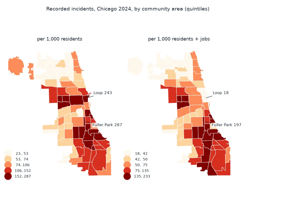
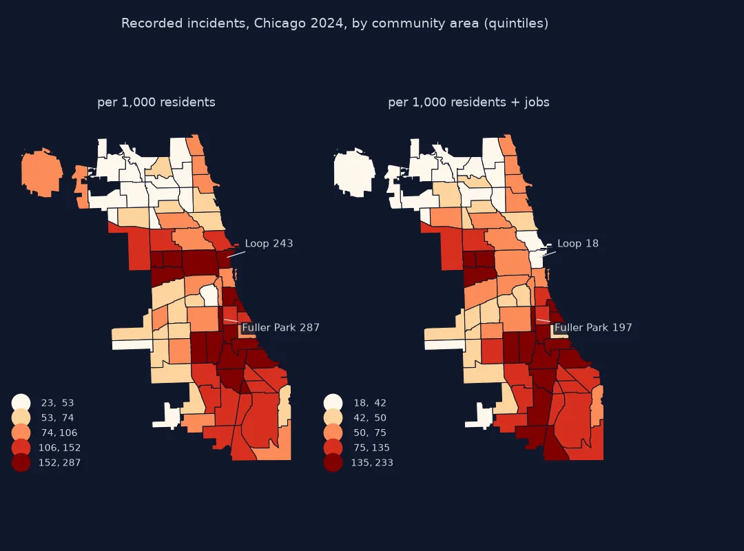
A map of crime counts by area mostly shows where people are. Dividing by population turns counts into rates, incidents per 1,000 residents, which can be compared between a dense neighbourhood and a sparse one. The division changes the map completely, and it brings its own problem: residents are not the only people an area's crime happens to. Downtown districts, with few residents and hundreds of thousands of workers, get rates that say more about the denominator than about danger.
This page counts Chicago's 2024 recorded incidents in the city's 77 community areas, divides by the city's own American Community Survey population estimates for each area, compares the ranking by count and by rate, and tries a second denominator that adds the jobs located in each area from the Census Bureau's LEHD data.
Quick answer
Count incidents per area with a spatial join, join a population table on the same area names, and divide:
n = gpd.sjoin(PTS, CA[["community", "geometry"]], predicate="within").groupby("community").size()
T = pd.DataFrame({"incidents": n, "residents": POP}).fillna(0)
T["per_1000"] = T.incidents / T.residents * 1000
print(f"city: {T.incidents.sum():,} incidents, {T.residents.sum():,.0f} residents, {T.incidents.sum() / T.residents.sum() * 1000:.1f} per 1,000")
print(T.sort_values("per_1000", ascending=False).head(5).round(1).to_string())
city: 256,654 incidents, 2,647,621 residents, 96.9 per 1,000
incidents residents per_1000
FULLER PARK 628 2186.0 287.3
ENGLEWOOD 5341 21337.0 250.3
LOOP 9286 38284.0 242.6
WEST GARFIELD PARK 3699 16345.0 226.3
GREATER GRAND CROSSING 6402 29052.0 220.4
Three of the top five are small or very small: Fuller Park has 2,186 residents, and its 628 incidents give the highest rate in the city. The Loop is third, with 38,284 residents.
Matching areas, count against rate rankings, workplace denominators
1. Check the two tables use the same areas
Counts and population must share a key. The city's ACS table names community areas in capitals, as the boundary file does; check that every name matches before dividing, because a mismatch gives a silent NaN:
print(f"in the boundaries but not the population table: {sorted(set(CA.community) - set(POP.index)) or 'none'}")
print(f"in the population table but not the boundaries: {sorted(set(POP.index) - set(CA.community)) or 'none'}")
print(f"population total {POP.sum():,.0f}; smallest area {POP.idxmin().title()} with {POP.min():,.0f}")
in the boundaries but not the population table: none
in the population table but not the boundaries: none
population total 2,647,621; smallest area Fuller Park with 2,186
2. Compare the ranking by count and by rate
T["rank_count"] = T.incidents.rank(ascending=False).astype(int)
T["rank_rate"] = T.per_1000.rank(ascending=False).astype(int)
moved = (T.rank_count - T.rank_rate).abs()
print(f"Spearman correlation of count and rate: {T.incidents.corr(T.per_1000, method='spearman'):.2f}")
print(f"areas moving 20 or more places: {(moved >= 20).sum()} of {len(T)}")
print(T.loc[["AUSTIN", "NEAR NORTH SIDE", "FULLER PARK", "ENGLEWOOD"], ["incidents", "residents", "per_1000", "rank_count", "rank_rate"]].round(1).to_string())
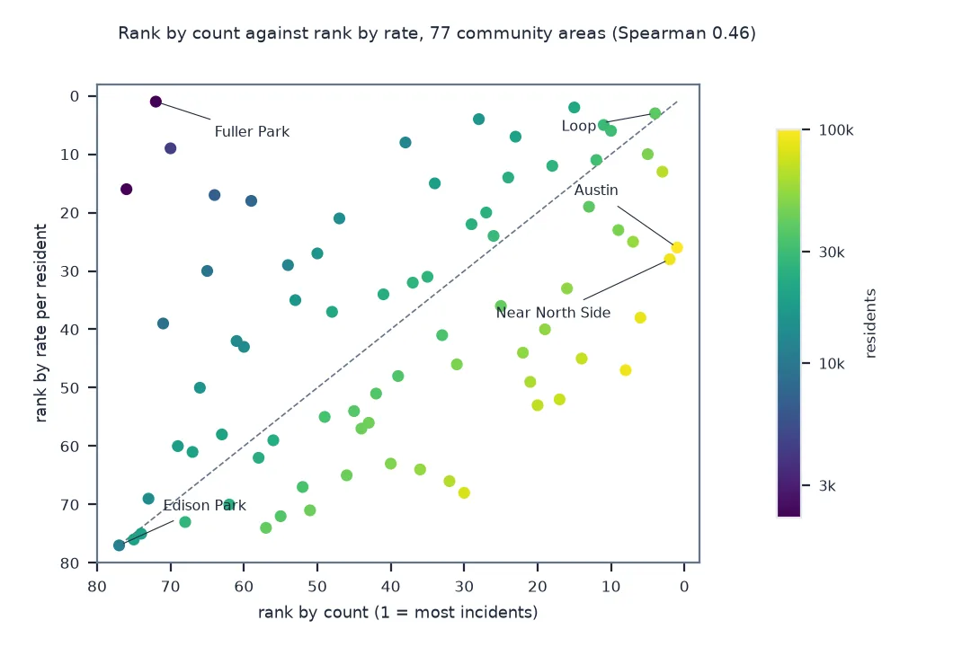
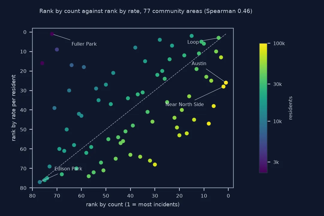
Spearman correlation of count and rate: 0.46
areas moving 20 or more places: 27 of 77
incidents residents per_1000 rank_count rank_rate
AUSTIN 12732 100278.0 127.0 1 26
NEAR NORTH SIDE 11400 91635.0 124.4 2 28
FULLER PARK 628 2186.0 287.3 72 1
ENGLEWOOD 5341 21337.0 250.3 15 2
Count and rate agree only loosely, with a rank correlation of 0.46. Austin, first by count, is 26th per resident because 100,278 people live there; Fuller Park goes from 72nd to first.
3. Add a workplace denominator
The Loop has 38,284 residents and far more people in it on a working day. LODES workplace area characteristics count jobs by census block; the crosswalk gives each block's internal point, so jobs can be summed by community area like the incidents:
g = gpd.GeoDataFrame(JOBS, geometry=gpd.points_from_xy(JOBS.blklondd, JOBS.blklatdd), crs=4326)
jobs = gpd.sjoin(g, CA[["community", "geometry"]], predicate="within").groupby("community").C000.sum()
T["jobs"] = jobs.reindex(T.index).fillna(0)
T["per_1000_res_jobs"] = T.incidents / (T.residents + T.jobs) * 1000
T["rank_res_jobs"] = T.per_1000_res_jobs.rank(ascending=False).astype(int)
print(f"jobs in community areas: {T.jobs.sum():,.0f}")
print(T.loc[["LOOP", "NEAR NORTH SIDE", "NEAR WEST SIDE", "ENGLEWOOD"], ["residents", "jobs", "per_1000", "per_1000_res_jobs", "rank_rate", "rank_res_jobs"]].round(1).to_string())
jobs in community areas: 1,410,516
residents jobs per_1000 per_1000_res_jobs rank_rate rank_res_jobs
LOOP 38284.0 466764 242.6 18.4 3 77
NEAR NORTH SIDE 91635.0 203446 124.4 38.6 28 67
NEAR WEST SIDE 65370.0 151814 167.4 50.4 13 46
ENGLEWOOD 21337.0 1631 250.3 232.5 2 1
Adding 466,764 jobs to the Loop's denominator moves it from third to 77th, last in the city. Englewood, with 1,631 jobs, barely changes and becomes first. Areas with few jobs keep their ranks; business districts fall.
A rate for one offence
The data used on this page
The City of Chicago's Crimes - 2001 to Present (ijzp-q8t2) for incidents dated 2024; the city's ACS 5 Year Data by Community Area (t68z-cikk), 2019–2023 estimates apportioned from tracts by the city; the community area boundaries; and the Census Bureau's LODES 8 workplace area characteristics for Illinois, all jobs (S000, JT00), 2022, with its block crosswalk.
from pathlib import Path

import geopandas as gpd
import pandas as pd
import requests

Path("data").mkdir(exist_ok=True)
URL = "https://data.cityofchicago.org/resource/ijzp-q8t2.json"
F = Path("data/chicago_crimes_2024.parquet")
if not F.exists():
    rows, offset = [], 0
    while True:
        part = requests.get(URL, timeout=300, params={
            "$where": "year=2024", "$limit": 50_000, "$offset": offset, "$order": "id",
            "$select": "id,date,primary_type,arrest,domestic,community_area,latitude,longitude,location_description,block,updated_on"}).json()
        rows += part; offset += len(part)
        if len(part) < 50_000:
            break
    pd.DataFrame(rows).to_parquet(F)
LODES = "https://lehd.ces.census.gov/data/lodes/LODES8/il/"
SRC = {"chicago_community_areas.geojson": "https://data.cityofchicago.org/resource/igwz-8jzy.geojson?$limit=100",
       "il_wac_S000_JT00_2022.csv.gz": LODES + "wac/il_wac_S000_JT00_2022.csv.gz",
       "il_xwalk.csv.gz": LODES + "il_xwalk.csv.gz"}
for name, url in SRC.items():
    if not Path("data", name).exists():
        Path("data", name).write_bytes(requests.get(url, timeout=300).content)

c = pd.read_parquet(F).dropna(subset=["latitude", "longitude"])
PTS = gpd.GeoDataFrame(c, geometry=gpd.points_from_xy(c.longitude.astype(float), c.latitude.astype(float)), crs=4326)
CA = gpd.read_file("data/chicago_community_areas.geojson")
acs = pd.DataFrame(requests.get("https://data.cityofchicago.org/resource/t68z-cikk.json", timeout=120,
                                params={"acs_year": "2023", "$limit": 200}).json())
POP = acs.set_index("community_area").total_population.astype(float)
wac = pd.read_csv("data/il_wac_S000_JT00_2022.csv.gz", usecols=["w_geocode", "C000"], dtype={"w_geocode": str})
xw = pd.read_csv("data/il_xwalk.csv.gz", usecols=["tabblk2020", "cty", "blklatdd", "blklondd"], dtype={"tabblk2020": str, "cty": str})
JOBS = wac.merge(xw[xw.cty == "17031"], left_on="w_geocode", right_on="tabblk2020")       # Cook County blocks
print(f"{len(PTS):,} incidents with coordinates; {len(POP)} areas with population; {len(JOBS):,} Cook County blocks with jobs")
257,524 incidents with coordinates; 77 areas with population; 32,056 Cook County blocks with jobs
Example 1: a rate for one offence
The same steps work for any offence. Robbery rates, with the count each rate rests on:
rob = gpd.sjoin(PTS[PTS.primary_type == "ROBBERY"], CA[["community", "geometry"]], predicate="within").groupby("community").size()
R = pd.DataFrame({"robberies": rob, "residents": POP}).fillna(0)
R["per_10000"] = R.robberies / R.residents * 10_000
print(f"city: {R.robberies.sum() / R.residents.sum() * 10_000:.1f} robberies per 10,000 residents")
print(R.sort_values("per_10000", ascending=False).head(4).round(1).to_string())
print(R.sort_values("per_10000").head(3).round(1).to_string())
city: 34.2 robberies per 10,000 residents
robberies residents per_10000
FULLER PARK 44 2186.0 201.3
ENGLEWOOD 233 21337.0 109.2
WEST GARFIELD PARK 177 16345.0 108.3
NORTH LAWNDALE 305 30355.0 100.5
robberies residents per_10000
MOUNT GREENWOOD 4 19107.0 2.1
EDISON PARK 3 11398.0 2.6
FOREST GLEN 7 19763.0 3.5
The highest robbery rate, Fuller Park's 201 per 10,000, rests on 44 robberies; the lowest rest on three to seven. At Edison Park's three, each robbery more or fewer moves the rate by a third.
A rate exists for comparison
A rate is a count divided by the population at risk, scaled to a readable unit. Its point is comparison: two areas with the same count and a fivefold difference in population are not equally affected. For crime, though, the population at risk is not fixed. Burglary happens to homes, so residents or households are the right denominator. Theft, robbery and assault happen to people wherever they are, which during the day is offices, shops and transit stations. A residential rate in a business district divides crimes against workers, shoppers and visitors by the few people who sleep there.
The jobs-based denominator is a crude correction, and it should be described as one. It double-counts residents who work in their own area, leaves out shoppers, tourists and students, and uses workplace counts from 2022 against crimes from 2024. What it shows is how sensitive the ranking is: the Loop goes from third to last. Where it matters, use more than one denominator and show both, rather than choosing the one that makes the map look the way you expect.
Small populations add a second problem. A handful of incidents in an area of two thousand people moves the rate by much more than the same number in an area of fifty thousand, so the top of a rate ranking tends to be filled by small areas. The rate on its own does not show this; print the count beside it.
Apportionment, ACS uncertainty and stray points
- Areal apportionment: the city's ACS table apportions tract estimates by area share, and its total is 0.6% below the city's ACS figure; that is the denominator's own error.
- ACS uncertainty: five-year estimates have margins of error, larger for small areas; the table does not include them.
- Years: the population is a 2019–2023 average; the incidents are 2024. Keep the mismatch small and state it.
- Units: per 1,000 suits all incidents; per 10,000 or 100,000 suits rarer offences, so rates stay above 1.
- Points outside every area: incidents at the city's edges or on the lake can miss a boundary file; count them.
Internal links
- How to download and map city crime data in Python — the incidents
- How to map commuting flows from LEHD LODES in Python — more on LODES
- How to map crime hotspots with kernel density in Python — density without areas
FAQ
How do I calculate a crime rate in Python?
Count incidents per area with geopandas.sjoin and groupby().size(), join a population table on the same area key, and compute count / population * 1000.
Why does the downtown area have such a high crime rate?
Because few people live there and many work or visit; residential population understates the people at risk. Chicago's Loop ranks third per resident and last per resident plus job.
Should I map crime counts or rates?
Rates for comparing areas of different sizes, with the counts shown beside them; counts for planning where incidents happen.
What population should I use for a crime rate?
The population exposed to that crime: residents or households for burglary, and some measure of people present, such as residents plus workers, for street crime.