
How to Map Superfund Sites by County
On this page
Problem statement
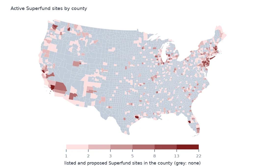
Where are the Superfund sites? Counted by state, the answer is New Jersey; counted by county, it is Silicon Valley, Los Angeles and the suburbs of Philadelphia and New York. The National Priorities List gives each site a county name, but names repeat across states, so the reliable county count comes from a spatial join of the site points to county boundaries. This page joins the active sites, those listed or proposed, to counties, ranks counties and states by count, area and population, and adds the deleted sites to show where cleanup has finished.
Quick answer
Join the listed and proposed sites to the 2024 county boundaries and count per county:
counties = gpd.read_file("data/cb_2024_us_county_20m.zip")
active = npl[npl.Status.isin(["NPL Site", "Proposed NPL Site"])]
j = gpd.sjoin(active.to_crs(counties.crs), counties[["GEOID", "NAMELSAD", "STUSPS", "geometry"]], how="left", predicate="within")
per = j.groupby(["GEOID", "NAMELSAD", "STUSPS"]).size().rename("sites").sort_values(ascending=False)
print(f"active sites: {len(active):,}; in a county: {j.GEOID.notna().sum():,}; counties with one: {len(per):,} of {len(counties):,}")
print(per.head(6).to_string())
active sites: 1,374; in a county: 1,364; counties with one: 670 of 3,222
GEOID NAMELSAD STUSPS
06085 Santa Clara County CA 21
06037 Los Angeles County CA 18
42091 Montgomery County PA 16
36059 Nassau County NY 14
48201 Harris County TX 13
34023 Middlesex County NJ 13
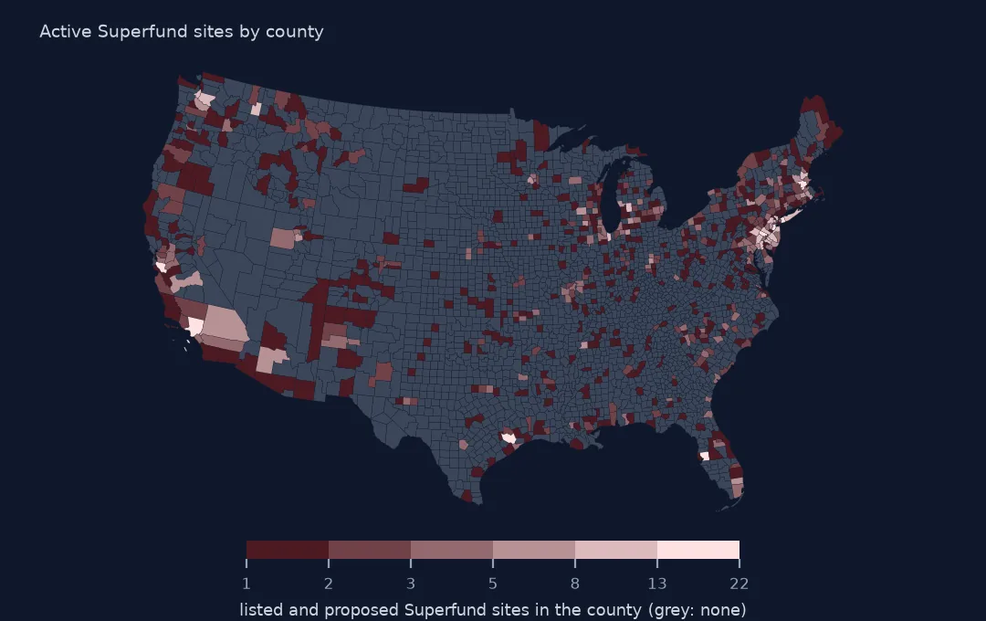
1,374 sites are listed or proposed, and 1,364 fall in a county; the other 10 are in Guam and the Virgin Islands, outside the boundary file, or on coasts and lakeshores where the generalised outlines miss the point. They lie in 670 of the 3,222 counties. Santa Clara County, California, has the most, 21, most of them the electronics and semiconductor plants of Silicon Valley, from Fairchild and Intel to Advanced Micro Devices, then Los Angeles County with 18 and Montgomery County, Pennsylvania, with 16.
States, area and population
1. By state
s = j.groupby("STUSPS").size().sort_values(ascending=False)
print(s.head(6).to_string())
print(f"states with none: {sorted(set(counties.STUSPS) - set(s.index))}")
STUSPS
NJ 115
CA 98
PA 93
NY 81
MI 67
TX 56
states with none: ['ND']
New Jersey has 115 active sites, California 98, Pennsylvania 93 and New York 81. North Dakota is the only state with none. The ranking follows industrial history more than size: New Jersey has a twentieth of California's area and more sites.
2. Per area
area = counties.to_crs(5070).set_index("STUSPS").area.groupby(level=0).sum() / 1e10   # per 10,000 km²
dens = (s / area.reindex(s.index)).sort_values(ascending=False)
print(dens.head(6).round(2).to_string())
STUSPS
NJ 56.97
DC 55.89
RI 37.45
DE 33.81
PR 19.31
MA 15.04
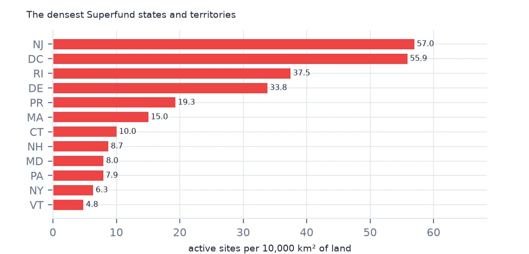
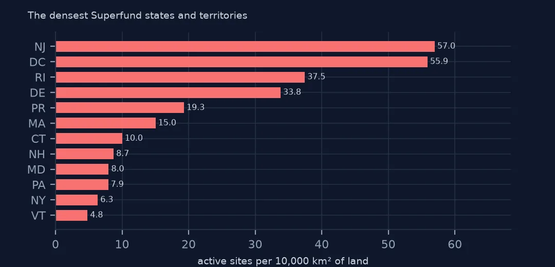
Per 10,000 km² of land, New Jersey has 56.97 active sites and DC 55.89, then Rhode Island, Delaware, Puerto Rico and Massachusetts. Small, old, industrial places are the densest, and the western states, with sites spread over huge areas, the sparsest.
3. Per resident
pop = pd.read_csv(Z.open("co-est2024-alldata.csv"), encoding="latin-1", dtype={"STATE": str, "COUNTY": str})
pop = pop[pop.SUMLEV == 50].assign(GEOID=lambda d: d.STATE + d.COUNTY).set_index("GEOID").POPESTIMATE2024
c = per.reset_index().set_index("GEOID").join(pop.rename("pop"))
c["per_100k"] = c.sites / c["pop"] * 1e5
print(c[c["pop"] >= 100_000].nlargest(5, "per_100k")[["NAMELSAD", "STUSPS", "sites", "pop", "per_100k"]].round(1).to_string())
NAMELSAD STUSPS sites pop per_100k
GEOID
24015 Cecil County MD 5 106305.0 4.7
26121 Muskegon County MI 7 177428.0 3.9
42001 Adams County PA 4 107914.0 3.7
18039 Elkhart County IN 7 207436.0 3.4
33017 Strafford County NH 4 134202.0 3.0
Per resident, among counties of 100,000 people or more, Cecil County, Maryland, has 4.7 active sites per 100,000 residents, Muskegon County, Michigan, 3.9, and Adams County, Pennsylvania, 3.7. These are mid-sized counties with a few large industrial or military sites, where the big metropolitan counties, with more sites in total, spread them over millions of people.
Deleted sites on the same map
The data used on this page
The US Environmental Protection Agency's Superfund National Priorities List (NPL) Sites with Status Information and its national Superfund site boundaries, every record of both ArcGIS layers, downloaded on 28 October 2026 and saved on this site, because EPA edits both as sites are proposed, listed, completed and deleted. Public domain. The contact names, telephone numbers and e-mail addresses of EPA staff in the boundary layer were left out of the copy. Tract centres of population are the Census Bureau's 2020 file, county populations its Vintage 2024 estimates and boundaries its 2024 cartographic files, all public domain.
from pathlib import Path
import zipfile

import geopandas as gpd
import numpy as np
import pandas as pd
import requests

Path("data").mkdir(exist_ok=True)
# EPA's Superfund National Priorities List with status information and EPA's Superfund site boundaries, with the
# Census Bureau's 2020 tract centres of population, 2024 county estimates, counties and states. Saved 28 October 2026:
# EPA updates both layers as sites are proposed, listed, completed and deleted.
# Live: https://services.arcgis.com/cJ9YHowT8TU7DUyn/arcgis/rest/services/Superfund_National_Priorities_List_(NPL)_Sites_with_Status_Information/FeatureServer/0
ARCHIVE = "epa-superfund-npl-2026-10-28.zip"
if not Path(f"data/{ARCHIVE}").exists():
    Path(f"data/{ARCHIVE}").write_bytes(requests.get(f"https://data.spatialworkflow.io/{ARCHIVE}", timeout=600).content)
Z = zipfile.ZipFile(f"data/{ARCHIVE}")
for f in ["npl-sites-status.geojson", "npl-site-boundaries.geojson", "cb_2024_us_county_20m.zip", "cb_2024_us_state_20m.zip"]:
    if not Path(f"data/{f}").exists():
        Path(f"data/{f}").write_bytes(Z.read(f))
npl = gpd.read_file("data/npl-sites-status.geojson")
npl = gpd.GeoDataFrame(npl.drop(columns="geometry"), geometry=gpd.points_from_xy(npl.Longitude, npl.Latitude), crs=4326)
DATES = ["Proposed_Date", "Listing_Date", "Construction_Completion_Date", "NOID_Date", "Deletion_Date"]
npl[DATES] = npl[DATES].apply(pd.to_datetime, format="%m/%d/%Y")        # stored as MM/DD/YYYY text
print(f"Superfund National Priorities List: {len(npl):,} sites, {npl.Status.value_counts().to_dict()}")
Superfund National Priorities List: 1,840 sites, {'NPL Site': 1337, 'Deleted NPL Site': 466, 'Proposed NPL Site': 37}
Example 1: deleted sites on the same map
d = npl[npl.Status == "Deleted NPL Site"]
jd = gpd.sjoin(d.to_crs(counties.crs), counties[["GEOID", "STUSPS", "geometry"]], how="left", predicate="within")
print(f"deleted sites: {len(d)}; their counties: {jd.GEOID.nunique()}; counties with only deleted sites: {len(set(jd.GEOID.dropna()) - set(j.GEOID.dropna()))}")
print(jd.STUSPS.value_counts().head(4).to_dict())
deleted sites: 466; their counties: 297; counties with only deleted sites: 120
{'NY': 39, 'NJ': 37, 'PA': 35, 'FL': 30}
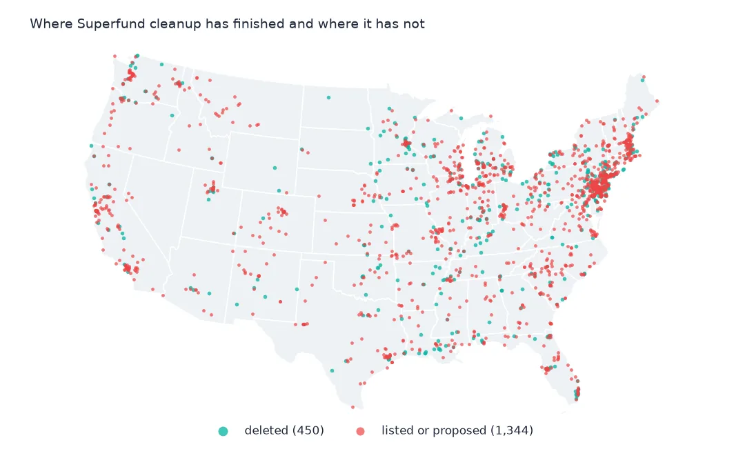
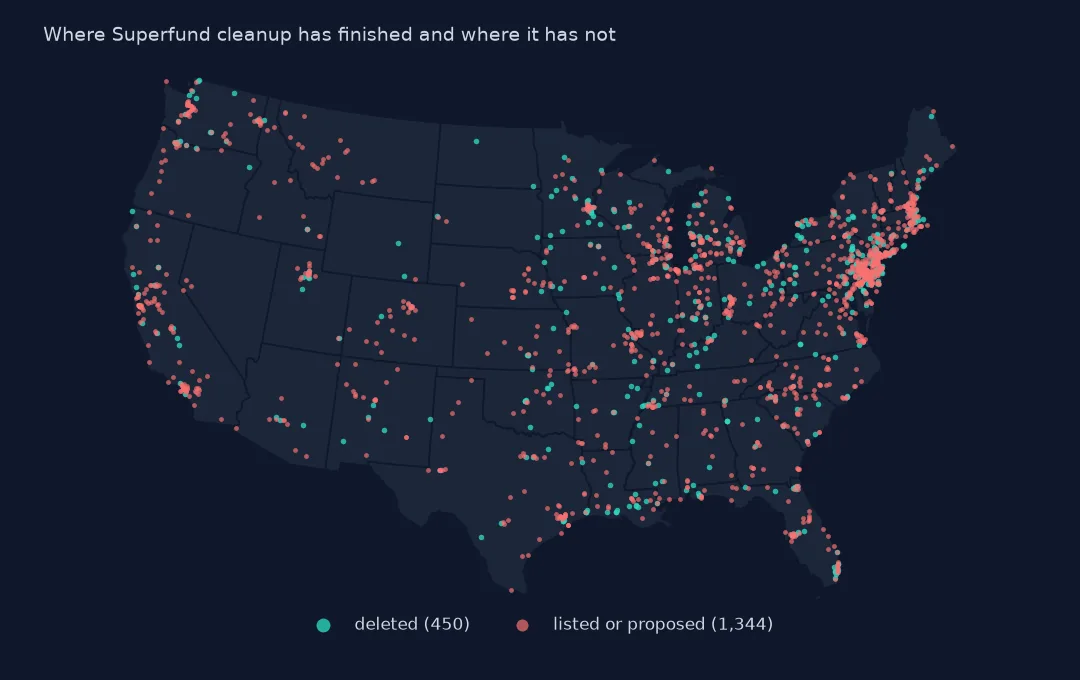
The 466 deleted sites are in 297 counties, and 120 of those counties have only deleted sites now: their Superfund history is over. New York, New Jersey, Pennsylvania and Florida have deleted the most. A map of active sites alone hides where cleanup has succeeded.
Internal links
- People near Superfund sites — distance instead of county counts
- Site boundaries — the outlines behind the points
- Reading the list — the status column used here
- Toxic releases by county — today's industrial pollution on the same map