
Age Standardisation Explained
On this page
Problem statement
Age standardisation is the most common adjustment in health statistics and one of the least understood. An age-standardised death rate of 726.5 per 100,000 for Florida is not the rate at which Floridians died, and choosing a different standard population would make it a different number. What standardisation does is replace each area's own age structure with a common one, so that the comparison between areas is about death rates at each age rather than about who lives there.
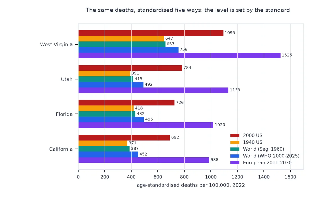
This page explains what the standard population does, using 2022 death rates for the 50 states and DC under five published standards: the 2000 and 1940 US standards, the World (Segi 1960) and WHO 2000–2025 world standards, and the 2011–2030 European standard. The levels change a lot. Most comparisons change little, but not all: Florida and Utah swap places.
Quick answer
An age-standardised rate is a weighted average of age-specific rates, and the standard population supplies the weights. Changing the weights changes the level:
rates = DEATHS.fillna(0) / POP * 1e5                                   # age-specific rates, per 100,000
adj = pd.DataFrame({name: rates.mul(w, axis=1).sum(axis=1) for name, w in WEIGHTS.items()})
print(adj.loc[["Florida", "Utah", "West Virginia"]].round(1).T.to_string())
state Florida Utah West Virginia
2000 US 726.5 783.7 1094.9
1940 US 418.0 390.8 646.9
World (Segi 1960) 431.5 415.4 657.1
World (WHO 2000-2025) 495.0 491.9 755.7
European 2011-2030 1019.7 1133.2 1525.0
A crude rate is a weighted average, and five standards
1. A crude rate is also a weighted average
The crude rate weights the same age-specific rates by the area's own population shares. That is the whole difference between crude and standardised rates:
own = POP.loc["Florida"] / POP.loc["Florida"].sum()
print(f"Florida: crude {(rates.loc['Florida'] * own).sum():.1f}, which equals deaths ÷ population "
      f"{DEATHS.loc['Florida'].sum() / POP.loc['Florida'].sum() * 1e5:.1f}")
print(f"weight on ages 65+: Florida's own {own[AGES[8:]].sum():.1%}, the 2000 US standard {WEIGHTS['2000 US'][AGES[8:]].sum():.1%}")
Florida: crude 1090.3, which equals deaths ÷ population 1090.3
weight on ages 65+: Florida's own 21.6%, the 2000 US standard 12.6%
2. The weights of the five standards
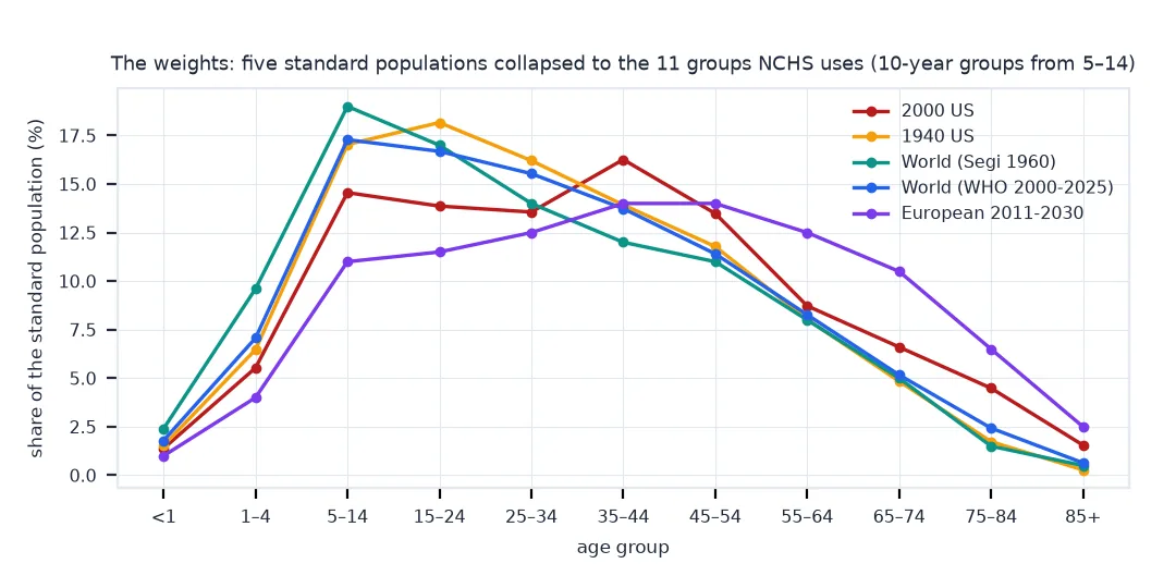
The standards differ most in how much weight they give to old ages, where death rates are highest:
W = pd.DataFrame(WEIGHTS)
print(pd.DataFrame({"under 15": W.loc[AGES[:3]].sum(), "15-64": W.loc[AGES[3:8]].sum(), "65+": W.loc[AGES[8:]].sum(),
                    "85+": W.loc[AGES[10]]}).map("{:.1%}".format).to_string())
under 15 15-64 65+ 85+
2000 US 21.5% 65.9% 12.6% 1.6%
1940 US 25.0% 68.1% 6.8% 0.3%
World (Segi 1960) 31.0% 62.0% 7.0% 0.5%
World (WHO 2000-2025) 26.1% 65.6% 8.2% 0.6%
European 2011-2030 16.0% 64.5% 19.5% 2.5%
3. The ranking mostly holds
Standards reorder areas only where their age-specific death rates differ in shape, for example high at young ages but low at old ones:
ranks = adj.rank(ascending=False)
print(f"rank correlation with the 2000 US standard: " + ", ".join(f"{c} {ranks[c].corr(ranks['2000 US']):.3f}" for c in ranks if c != "2000 US"))
moves = (ranks.max(axis=1) - ranks.min(axis=1))
print(f"largest range of ranks across standards: {moves.max():.0f} places ({moves.idxmax()}); median {moves.median():.0f}")
rank correlation with the 2000 US standard: 1940 US 0.973, World (Segi 1960) 0.981, World (WHO 2000-2025) 0.989, European 2011-2030 0.994
largest range of ranks across standards: 15 places (Alaska); median 2
Most states move a place or two. Florida and Utah show what makes a state move: Florida's death rates are higher than Utah's at most ages under 75 (by about 30% in the working ages) and lower at 75 and over, so a standard with many old people puts Florida below Utah and a young one puts it above:
print((rates.loc["Florida"] / rates.loc["Utah"]).round(2).to_string())age_group
Under 1 year 1.20
1-4 years 1.31
5-14 years 0.86
15-24 years 1.30
25-34 years 1.57
35-44 years 1.31
45-54 years 1.29
55-64 years 1.26
65-74 years 1.06
75-84 years 0.81
85 years and over 0.72
The national rate under each standard
The data used on this page
Deaths by state and age for 2022 from the CDC dataset Provisional COVID-19 Deaths by Sex and Age (all causes; New York City added into New York), Vintage 2022 state population estimates by age, and the standard populations distributed by SEER, in 19 age groups. Each standard's code in the SEER file was matched to the published tables by its values.
from pathlib import Path

import numpy as np
import pandas as pd
import requests

Path("data").mkdir(exist_ok=True)
SRC = {"sc-est2022-alldata6.csv": "https://www2.census.gov/programs-surveys/popest/datasets/2020-2022/state/asrh/sc-est2022-alldata6.csv",
       "stdpop.19ages.txt": "https://seer.cancer.gov/stdpopulations/stdpop.19ages.txt"}
for name, url in SRC.items():
    if not Path("data", name).exists():
        Path("data", name).write_bytes(requests.get(url, timeout=300).content)

AGES = ["Under 1 year", "1-4 years", "5-14 years", "15-24 years", "25-34 years", "35-44 years",
        "45-54 years", "55-64 years", "65-74 years", "75-84 years", "85 years and over"]
EDGES = [0, 1, 5, 15, 25, 35, 45, 55, 65, 75, 85]
api = pd.DataFrame(requests.get("https://data.cdc.gov/resource/9bhg-hcku.json", params={
    "$where": "`group` = 'By Year' AND year = '2022' AND sex = 'All Sexes'",
    "$select": "state, age_group, total_deaths", "$limit": 5000}, timeout=120).json())
api["state"] = api.state.replace({"New York City": "New York"})
api["deaths"] = api.total_deaths.astype(float)
DEATHS = (api[api.age_group.isin(AGES)].groupby(["state", "age_group"]).deaths.sum(min_count=1)
             .unstack()[AGES].drop(index=["United States", "Puerto Rico"]))
p = pd.read_csv("data/sc-est2022-alldata6.csv")
p = p[(p.SUMLEV == 40) & (p.SEX == 0) & (p.ORIGIN == 0)].groupby(["NAME", "AGE"]).POPESTIMATE2022.sum().unstack()
POP = p.T.groupby(np.searchsorted(EDGES, p.columns, side="right") - 1).sum().T.set_axis(AGES, axis=1).loc[DEATHS.index]

std = pd.read_fwf("data/stdpop.19ages.txt", widths=[3, 3, 8], names=["standard", "age", "pop"], dtype={"standard": str})
CODES = {"2000 US": "201", "1940 US": "141", "World (Segi 1960)": "006", "World (WHO 2000-2025)": "010", "European 2011-2030": "014"}
WEIGHTS = {}
for name, code in CODES.items():
    s = std[std.standard == code]["pop"].to_numpy()                   # 19 groups: 0, 1–4, 5–9, ..., 85+
    WEIGHTS[name] = pd.Series(np.add.reduceat(s, [0, 1, 2, 4, 6, 8, 10, 12, 14, 16, 18]) / s.sum(), index=AGES)
print(f"{len(DEATHS)} areas; standards: {', '.join(f'{n} ({std[std.standard == c].age.nunique()} groups)' for n, c in CODES.items())}")
51 areas; standards: 2000 US (19 groups), 1940 US (19 groups), World (Segi 1960) (19 groups), World (WHO 2000-2025) (19 groups), European 2011-2030 (19 groups)
Example 1: the national rate under each standard
us = DEATHS.fillna(0).sum() / POP.sum() * 1e5
print(pd.Series({n: (us * w).sum() for n, w in WEIGHTS.items()}).round(1).to_string())
print(f"crude rate: {DEATHS.sum().sum() / POP.sum().sum() * 1e5:.1f}")
2000 US 801.2
1940 US 441.6
World (Segi 1960) 458.6
World (WHO 2000-2025) 532.1
European 2011-2030 1137.7
crude rate: 986.8
The US population of 2022 is older than the 2000 standard, so its crude rate is above the standardised one. The world standards are younger and give much lower rates; the European standard is older and gives a higher one. International comparisons must use the same standard.
Example 2: comparing two states
The ratio of two standardised rates is much less sensitive to the standard than the rates themselves:
ratio = adj.loc["West Virginia"] / adj.loc["California"]
print(ratio.round(3).to_string())
2000 US 1.583
1940 US 1.746
World (Segi 1960) 1.697
World (WHO 2000-2025) 1.673
European 2011-2030 1.543
A standardised rate answers a hypothetical
A standardised rate answers a hypothetical question: how many deaths per 100,000 would this area have if its people had the standard population's ages but kept their own death rates at each age? The answer is a weighted average of the area's age-specific rates, and since death rates at old ages are a hundred times those of young adults, the weight the standard gives to old ages decides the level. A standard with many old people, such as the European 2011–2030 one, gives high rates; a young world standard gives low ones.
The comparisons between areas are much more stable. If one state's death rates are higher than another's at every age, it is higher under every standard. Only where the two states' age patterns cross can a standard reorder them. Among US states the median state's rank moves by 2 places across the five standards, and Alaska's by 15. That is why the choice of standard is mostly a convention: NCHS and most US agencies use the 2000 US standard, the World Health Organization uses its world standard, and Eurostat the European one. Mixing rates from different conventions is the mistake to avoid.
Not a real rate, and one standard everywhere
- Not a real rate: a standardised rate is for comparison; for counts of deaths or the burden on services, use crude numbers.
- Same groups: a standard and the data must share age groups; collapse the standard's 19 groups to match, as here.
- Same standard everywhere: compare only rates standardised to the same population, and say which one.
- Sex: standardise by sex separately, or by age and sex together, where the data allow.
- Indirect standardisation: when deaths by age are not available, the standardised mortality ratio uses standard rates instead of a standard population.
Internal links
- How to calculate age-adjusted death rates in Python — the calculation, checked against NCHS
- Why does my death rate map just show where old people live? — the symptom, and the SMR
FAQ
What does age standardisation do?
It replaces each area's own age structure with a common standard population, so that rates differ only because of death rates at each age.
Why do age-standardised rates change with the standard population?
They are weighted averages of age-specific rates, and different standards give different weights, especially to old ages, where death rates are highest.
Which standard population should I use?
The one used by the figures you will compare with: the 2000 US standard for US data, the WHO world standard for international comparisons, the European standard for European data.
Is an age-standardised rate the real death rate?
No. It is a comparison figure; the crude rate is the actual number of deaths per person in the area.