
Why Does My Health Map Look Like a Poverty Map?
On this page
Problem statement
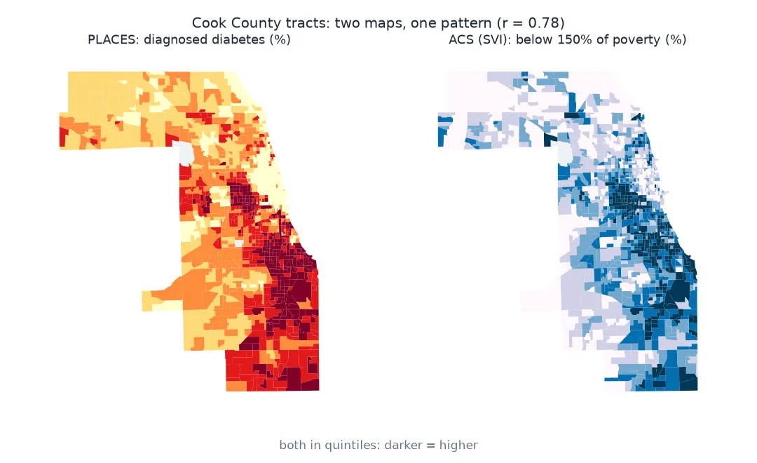
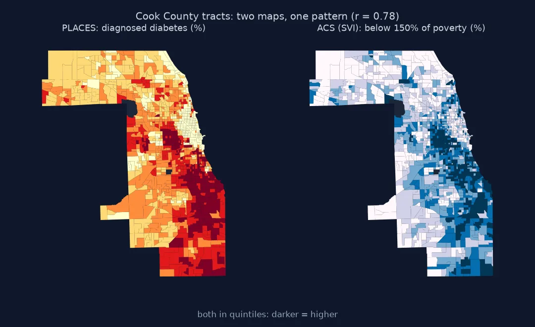
You map diabetes, obesity or smoking by census tract from CDC PLACES and the pattern is familiar: it is the map of poverty and race in the city. Then you regress the health estimate on poverty and find a strong relationship. Both results are largely built in. PLACES tract values are not measurements; they are predictions from a model whose inputs include each tract's age, sex and race/ethnicity make-up, applied to Census population counts. A map of the predictions is in large part a map of those inputs, and a regression of the predictions on demographics recovers the model.
This page measures how much of the variation in five PLACES measures across Cook County's tracts is accounted for by four Census demographic variables from the CDC Social Vulnerability Index (SVI), and maps what is left.
Quick answer
Regress the tract estimates on a few demographic variables and look at the share of variance explained:
X = np.column_stack([np.ones(len(M))] + [M[c] for c in DEMOG])
r2 = {}
for y in MEASURES:
    beta, *_ = np.linalg.lstsq(X, M[y], rcond=None)
    r2[y] = 1 - ((M[y] - X @ beta) ** 2).sum() / ((M[y] - M[y].mean()) ** 2).sum()
print(f"{len(M)} tracts; share of tract-to-tract variation explained by {', '.join(DEMOG)}:")
print(pd.Series(r2).sort_values(ascending=False).map("{:.0%}".format).to_string())
1328 tracts; share of tract-to-tract variation explained by EP_POV150, EP_AGE65, EP_MINRTY, EP_NOHSDP:
DIABETES 85%
OBESITY 82%
CSMOKING 80%
BINGE 78%
DEPRESSION 65%
Check the correlations, map the residual
1. Check the correlations
Start with the simple version: how closely does each health estimate follow poverty and the share of residents from racial and ethnic minorities?
print(M[DEMOG + MEASURES].corr().loc[["EP_POV150", "EP_MINRTY", "EP_AGE65"], MEASURES].round(2).to_string()) DIABETES OBESITY CSMOKING DEPRESSION BINGE
EP_POV150 0.78 0.83 0.87 0.01 -0.60
EP_MINRTY 0.79 0.85 0.74 -0.45 -0.66
EP_AGE65 0.25 -0.04 -0.02 -0.39 -0.45
Correlations of 0.8 between an outcome and a predictor would be remarkable in survey data for individuals. Between model predictions and the model's inputs they are expected.
2. Map the residual, not the estimate
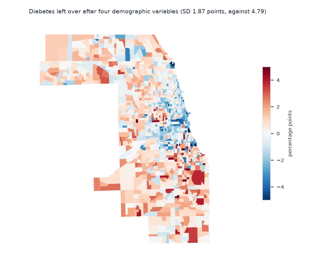
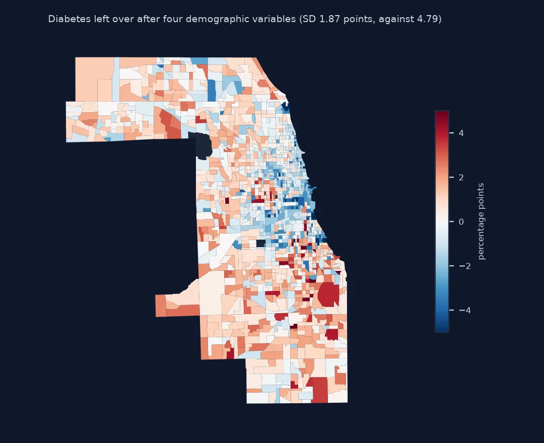
The part of each estimate not accounted for by the demographic variables is where PLACES says something the demographics alone would not:
beta, *_ = np.linalg.lstsq(X, M["DIABETES"], rcond=None)
M["resid"] = M["DIABETES"] - X @ beta
print(f"diabetes estimates: SD {M['DIABETES'].std():.2f} points; residual after demographics: SD {M['resid'].std():.2f} points")
print(f"tracts with a residual beyond ±2 points: {(M.resid.abs() > 2).sum()} of {len(M)}")
diabetes estimates: SD 4.79 points; residual after demographics: SD 1.87 points
tracts with a residual beyond ±2 points: 315 of 1328
3. Do not use the estimates as an outcome for demographics
A study of "poverty and diabetes" using PLACES tract estimates mostly measures the model's coefficients. Compare one variable's apparent effect with the model:
slope = np.polyfit(M["EP_POV150"], M["DIABETES"], 1)[0]
print(f"apparent effect: +{slope * 10:.2f} points of diabetes per 10 points of poverty (r = {M['EP_POV150'].corr(M['DIABETES']):.2f})")
print("this is a property of the estimates, which were predicted partly from these same characteristics")
apparent effect: +2.42 points of diabetes per 10 points of poverty (r = 0.78)
this is a property of the estimates, which were predicted partly from these same characteristics
The exception that proves the rule
The data used on this page
CDC PLACES census tract estimates (2025 release, survey year 2023) for Cook County, Illinois, from data.cdc.gov (cwsq-ngmh), and the CDC/ATSDR Social Vulnerability Index 2022 for Illinois, whose EP_ variables are American Community Survey 2018–2022 percentages by tract.
from pathlib import Path

import numpy as np
import pandas as pd
import requests

Path("data").mkdir(exist_ok=True)
F = Path("data/svi_2022_illinois.csv")
if not F.exists():
    F.write_bytes(requests.get("https://svi.cdc.gov/Documents/Data/2022/csv/states/Illinois.csv", timeout=300).content)
svi = pd.read_csv(F, dtype={"FIPS": str})
svi = svi[svi.FIPS.str.startswith("17031")].set_index("FIPS")
MEASURES = ["DIABETES", "OBESITY", "CSMOKING", "DEPRESSION", "BINGE"]
places = pd.DataFrame(requests.get("https://data.cdc.gov/resource/cwsq-ngmh.json",
                                   params={"$where": f"countyfips = '17031' AND measureid in ({', '.join(repr(m) for m in MEASURES)})",
                                           "$select": "locationname, measureid, data_value", "$limit": 20000}, timeout=120).json())
wide = places.pivot(index="locationname", columns="measureid", values="data_value").astype(float)
DEMOG = ["EP_POV150", "EP_AGE65", "EP_MINRTY", "EP_NOHSDP"]          # below 150% poverty, 65+, minority, no high-school diploma
M = svi[DEMOG].replace(-999, np.nan).join(wide, how="inner").dropna()
print(f"{len(svi)} SVI tracts, {len(wide)} PLACES tracts, {len(M)} with both")
1331 SVI tracts, 1328 PLACES tracts, 1328 with both
Example 1: the exception that proves the rule
print(f"depression vs minority share: r = {M['DEPRESSION'].corr(M['EP_MINRTY']):.2f}; binge drinking vs poverty: r = {M['BINGE'].corr(M['EP_POV150']):.2f}")depression vs minority share: r = -0.45; binge drinking vs poverty: r = -0.60
Not every measure follows poverty upwards. Depression is estimated higher where the share of minority residents is lower, and binge drinking where poverty is lower, because that is what the survey shows for individuals with those characteristics; the model carries the individual-level pattern to the tracts.
Small area estimates come from a demographic model
Small area estimates exist because surveys are too small to measure every tract directly. PLACES fits a multilevel regression to the Behavioral Risk Factor Surveillance System (BRFSS), using individuals' age, sex and race/ethnicity along with county and state effects, and then predicts for every tract by weighting those predictions with its population. Much of the variation between tracts within a county therefore comes from differences in their population make-up. Poverty and education are strongly correlated with that make-up, so they explain the estimates almost as well as the inputs themselves.
None of this makes PLACES wrong. Where tracts differ mainly in composition, the estimates show what that composition implies, which is valuable for planning. It does mean that the map adds less independent information than its detail suggests, and that relationships between PLACES estimates and demographics cannot be read as evidence. For questions about causes, use individual survey data or measured outcomes, such as hospital records or vital statistics.
County effects and what R-squared is not
- County effects: within one county the county effect is constant; across counties, it adds variation not explained by demographics.
- Variables: SVI
EP_values are ACS estimates with their own margins of error; small tracts are noisy on both sides. - R² is not a test: a high R² against demographics is expected by construction, not a finding.
- Other PLACES uses: comparing counties, tracking a measure over releases, or targeting outreach remain sensible uses.
- SVI missing values are coded −999; replace them before analysis.
Internal links
- How to map CDC PLACES health estimates by census tract — the data
- The ecological fallacy explained — what area-level relationships do not say about people
FAQ
Why do PLACES health estimates correlate so strongly with poverty?
They are model predictions from each tract's demographic composition, and poverty is strongly correlated with that composition.
Can I regress PLACES estimates on demographic variables?
You can, but the result largely reproduces the model that made the estimates; it is not independent evidence of a relationship.
Are PLACES estimates useful at all?
Yes, for showing broad patterns, planning and outreach, as long as they are not treated as measurements of each tract.
What is the CDC Social Vulnerability Index?
A tract-level index from the CDC and ATSDR built from American Community Survey variables such as poverty, age, disability, housing and language; the EP_ columns hold the underlying percentages.