Why Does My Death Rate Map Just Show Where Old People Live?

Problem statement

You divide deaths by population for each area, map the result, and the darkest areas are retirement destinations and places young people have left. The map is right about the number of deaths per person, and it answers a different question from the one most readers ask. Among adults, death rates rise roughly tenfold every 30 years of age (in 2022, from 258 per 100,000 at 35–44 to 1,984 at 65–74), so a crude rate is dominated by how many old people an area has. To compare the health of places, the rates have to be standardised for age.

This page shows the symptom with 2022 death rates for the 50 states and DC, and fixes it with indirect standardisation, the method that works when you know only each area's total deaths, as is common for counties and smaller areas.

Quick answer

Compute the deaths each area would have at national age-specific rates, and divide the observed deaths by that expected number:

national_rate = DEATHS.sum() / POP.sum()                         # deaths per person in each age group
expected = POP.mul(national_rate, axis=1).sum(axis=1)
observed = TOTAL                                                 # all-ages deaths: no age breakdown needed
smr = observed / expected
print(f"standardised mortality ratio: {smr.min():.2f} ({smr.idxmin()}) to {smr.max():.2f} ({smr.idxmax()})")
print(smr.loc[["Florida", "Maine", "Texas", "Utah"]].round(2).to_string())

standardised mortality ratio: 0.77 (Hawaii) to 1.35 (West Virginia)
state
Florida    0.89
Maine      1.03
Texas      1.04
Utah       0.96

Check for an age map, read the ratio, check it

1. Check whether the map is an age map

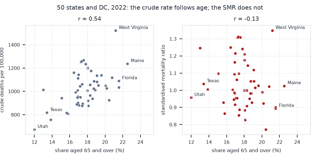
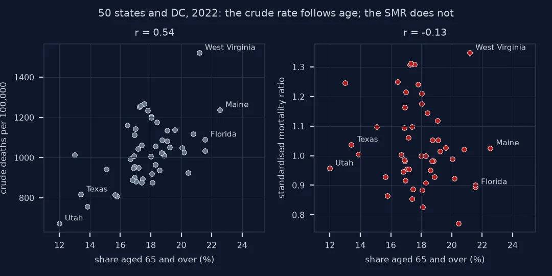
Correlate the crude rate with the share of people aged 65 and over. A strong correlation means the map mostly shows age:

old = POP[AGES[8:]].sum(axis=1) / POP.sum(axis=1)
crude = TOTAL / POP.sum(axis=1) * 1e5
print(f"crude rate against share aged 65+: r = {crude.corr(old):.2f}; standardised ratio against it: r = {smr.corr(old):.2f}")
print(f"Florida: {old['Florida']:.1%} aged 65+, crude {crude['Florida']:.0f} per 100,000; "
      f"Utah: {old['Utah']:.1%}, crude {crude['Utah']:.0f}")
print("national deaths per 100,000:", ", ".join(f"{a} {national_rate[a] * 1e5:,.0f}" for a in AGES[5:]))

crude rate against share aged 65+: r = 0.54; standardised ratio against it: r = -0.13
Florida: 21.6% aged 65+, crude 1090 per 100,000; Utah: 12.0%, crude 673
national deaths per 100,000: 35-44 years 258, 45-54 years 456, 55-64 years 997, 65-74 years 1,984, 75-84 years 4,715, 85 years and over 14,398

2. Read the ratio as "more or fewer deaths than expected"

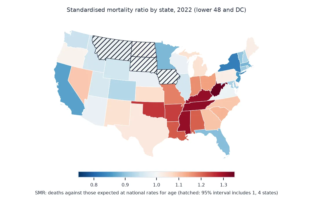
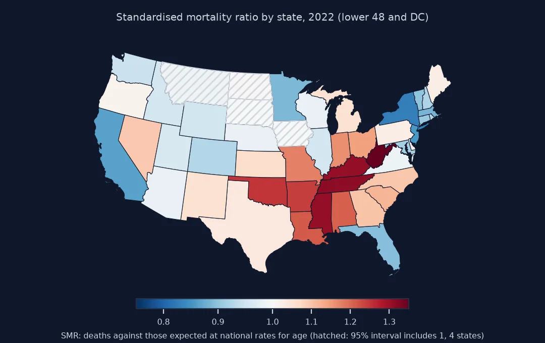
An SMR of 1.2 means 20% more deaths than the area's population would have at national rates, whatever its age structure. Its 95% interval comes from the Poisson distribution of the observed count:

from scipy.stats import chi2

lo = chi2.ppf(0.025, 2 * observed) / 2 / expected
hi = chi2.ppf(0.975, 2 * (observed + 1)) / 2 / expected
S = pd.DataFrame({"observed": observed, "expected": expected.round(0), "smr": smr, "lo": lo, "hi": hi}).round(3)
print(S.loc[["West Virginia", "Florida", "Utah", "Wyoming"]].to_string())
print(f"states with an interval entirely above 1: {(S.lo > 1).sum()}; entirely below: {(S.hi < 1).sum()}")

               observed  expected    smr     lo     hi
state                                                 
West Virginia   27013.0   20037.0  1.348  1.332  1.364
Florida        242537.0  271290.0  0.894  0.890  0.898
Utah            22767.0   23782.0  0.957  0.945  0.970
Wyoming          5455.0    5733.0  0.951  0.926  0.977
states with an interval entirely above 1: 24; entirely below: 22

3. Check it against direct standardisation

Where deaths by age are known, the directly age-adjusted rate is the alternative. The two should rank areas similarly:

adjusted = (DEATHS.fillna(0) / POP * 1e5).mul(W, axis=1).sum(axis=1)
print(f"rank correlation of SMR and the age-adjusted rate: {smr.rank().corr(adjusted.rank()):.3f}")
gap = (smr.rank() - adjusted.rank()).abs()
print(f"largest rank difference: {gap.max():.0f} places ({gap.idxmax()}); median {gap.median():.0f}")

rank correlation of SMR and the age-adjusted rate: 0.996
largest rank difference: 3 places (Alaska); median 1

An SMR from totals alone

The data used on this page

Deaths by state and age for 2022 from the CDC dataset Provisional COVID-19 Deaths by Sex and Age (all-cause total_deaths; New York City added back into New York), the Census Bureau's Vintage 2022 state population estimates by age, and the 2000 US standard population for comparison.

from pathlib import Path

import numpy as np
import pandas as pd
import requests

Path("data").mkdir(exist_ok=True)
SRC = {"sc-est2022-alldata6.csv": "https://www2.census.gov/programs-surveys/popest/datasets/2020-2022/state/asrh/sc-est2022-alldata6.csv",
       "stdpop.19ages.txt": "https://seer.cancer.gov/stdpopulations/stdpop.19ages.txt"}
for name, url in SRC.items():
    if not Path("data", name).exists():
        Path("data", name).write_bytes(requests.get(url, timeout=300).content)

AGES = ["Under 1 year", "1-4 years", "5-14 years", "15-24 years", "25-34 years", "35-44 years",
        "45-54 years", "55-64 years", "65-74 years", "75-84 years", "85 years and over"]
EDGES = [0, 1, 5, 15, 25, 35, 45, 55, 65, 75, 85]
api = pd.DataFrame(requests.get("https://data.cdc.gov/resource/9bhg-hcku.json", params={
    "$where": "`group` = 'By Year' AND year = '2022' AND sex = 'All Sexes'",
    "$select": "state, age_group, total_deaths", "$limit": 5000}, timeout=120).json())
api["state"] = api.state.replace({"New York City": "New York"})
api["deaths"] = api.total_deaths.astype(float)
TOTAL = api[api.age_group == "All Ages"].groupby("state").deaths.sum().drop(["United States", "Puerto Rico"])
DEATHS = api[api.age_group.isin(AGES)].groupby(["state", "age_group"]).deaths.sum(min_count=1).unstack()[AGES].loc[TOTAL.index]

p = pd.read_csv("data/sc-est2022-alldata6.csv")
p = p[(p.SUMLEV == 40) & (p.SEX == 0) & (p.ORIGIN == 0)].groupby(["NAME", "AGE"]).POPESTIMATE2022.sum().unstack()
POP = p.T.groupby(np.searchsorted(EDGES, p.columns, side="right") - 1).sum().T.set_axis(AGES, axis=1).loc[TOTAL.index]
std = pd.read_fwf("data/stdpop.19ages.txt", widths=[3, 3, 8], names=["standard", "age", "pop"], dtype={"standard": str})
s = std[std.standard == "201"]["pop"].to_numpy()
W = pd.Series(np.add.reduceat(s, [0, 1, 2, 4, 6, 8, 10, 12, 14, 16, 18]) / s.sum(), index=AGES)
print(f"{len(TOTAL)} areas; {TOTAL.sum():,.0f} deaths; {POP.sum().sum():,} people")

51 areas; 3,288,942 deaths; 333,287,557 people

Example 1: the SMR needs only totals

The quick answer never used the deaths by age for each state, only the national age-specific rates. That is what makes it usable for counties, where deaths by age are often suppressed:

cells = DEATHS.isna().sum().sum()
print(f"suppressed age cells in the state data: {cells}; the SMR used none of them")

suppressed age cells in the state data: 6; the SMR used none of them

Example 2: what the crude map would have said

both = pd.DataFrame({"crude_rank": crude.rank(ascending=False), "smr_rank": smr.rank(ascending=False)}).astype(int)
both["moved"] = both.crude_rank - both.smr_rank
print(both.reindex(both.moved.abs().sort_values(ascending=False).index).head(6).to_string())

                      crude_rank  smr_rank  moved
state                                            
Florida                       16        45    -29
Texas                         47        20     27
Alaska                        50        25     25
Georgia                       37        14     23
District of Columbia          28         6     22
Vermont                       24        44    -20

Direct and indirect standardisation

Direct and indirect standardisation answer slightly different questions. Direct standardisation applies each area's age-specific rates to one standard population, so it needs deaths by age in every area, and its results can be compared with each other and with published rates on the same standard. Indirect standardisation applies one set of standard rates, usually national, to each area's own population, so it needs only total deaths. Its result, the SMR, compares each area with the standard, and strictly two SMRs compare areas only as far as their age structures are similar. In practice the two methods rank the states almost identically here.

The fix is not always standardisation. If the question is about burden, such as how many hospital beds or hospice places an area needs, the crude rate and the count are the right measures, and the old populations are the point. Standardise when the question is whether people in one place are less healthy than in another.

Small areas, standard rates and sex

• Small areas: SMRs of areas with few expected deaths have wide intervals; map the interval, or smooth them (see small area rates explained).
• The standard rates: national rates are the usual choice; another set of standard rates changes the SMRs and can reorder areas with unusual age structures, so say which you used.
• Age groups: use groups fine enough at old ages (75–84, 85+); one 65+ group leaves much of the age effect in.
• Sex: standardise by age and sex together where both are available.
• Residence and occurrence: death counts by place of occurrence put deaths in hospital counties; use counts by place of residence.

Internal links

• How to calculate age-adjusted death rates in Python — direct standardisation step by step
• Age standardisation explained — what the standard population does

FAQ

Why are death rates highest where older people live?

Death rates rise steeply with age, so an area's crude rate depends heavily on how many of its residents are old.

What is a standardised mortality ratio (SMR)?

Observed deaths divided by the deaths expected if the area had national age-specific rates; above 1 means more deaths than expected for its age structure.

When should I use an SMR instead of an age-adjusted rate?

When you know only total deaths for each area, not deaths by age, which is common for counties and smaller areas.

Is the crude death rate ever the right measure?

Yes, for questions of burden and service planning, where the number of deaths an area actually has is what matters.