
How to Calculate Age-Adjusted Death Rates in Python
On this page
Problem statement
CDC's provisional death counts for 2022 come by state and in the 11 age groups NCHS adjusts with — but with New York City reported apart from the rest of New York State, and every count from 1 to 9 suppressed. Turning them into age-adjusted rates means dividing each age group's deaths by its Census population, weighting the rates by the 2000 US standard population, and adding them up; the national result, 801.2 per 100,000, can then be checked against the 798.8 NCHS published. Florida's crude rate of 1,090 is a reminder of why: 22% of Floridians are 65 or over, against 13% of Texans.
This page computes crude and age-adjusted death rates for the 50 states and DC in 2022 from CDC death counts, Census population estimates and the 2000 US standard population, and checks the national result against the published NCHS figure.
Quick answer
Compute the age-specific rates, weight them by the standard population's age shares, and add them up:
def age_adjusted(deaths, pop, weights):
    """Direct standardisation: deaths and pop are areas × age groups; weights sum to 1."""
    return (deaths / pop * 1e5).mul(weights, axis=1).sum(axis=1)

crude = DEATHS.sum(axis=1) / POP.sum(axis=1) * 1e5
adjusted = age_adjusted(DEATHS.fillna(0), POP, W)
R = pd.DataFrame({"crude": crude, "adjusted": adjusted}).round(1)
R["rank_crude"] = R.crude.rank(ascending=False).astype(int)
R["rank_adjusted"] = R.adjusted.rank(ascending=False).astype(int)
print(R.loc[["West Virginia", "Florida", "Maine", "Texas", "Alaska", "Utah"]].to_string())
crude adjusted rank_crude rank_adjusted
state
West Virginia 1521.7 1094.9 1 1
Florida 1090.3 726.5 16 43
Maine 1237.4 833.5 5 20
Texas 817.3 830.1 47 22
Alaska 756.6 798.5 50 28
Utah 673.4 783.7 51 33
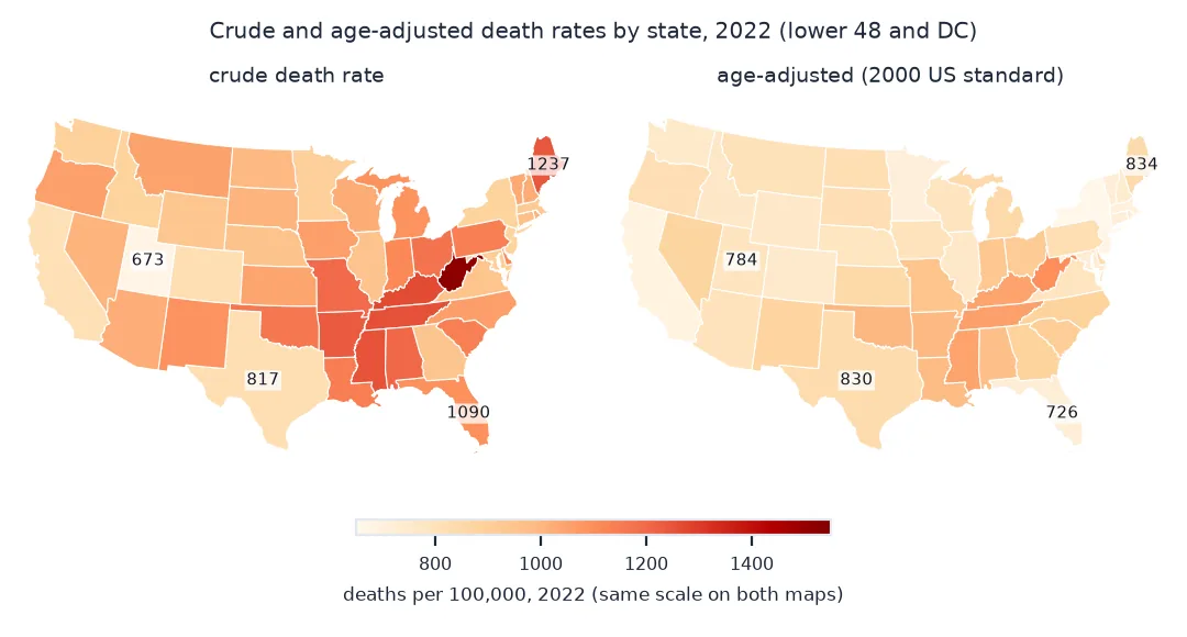
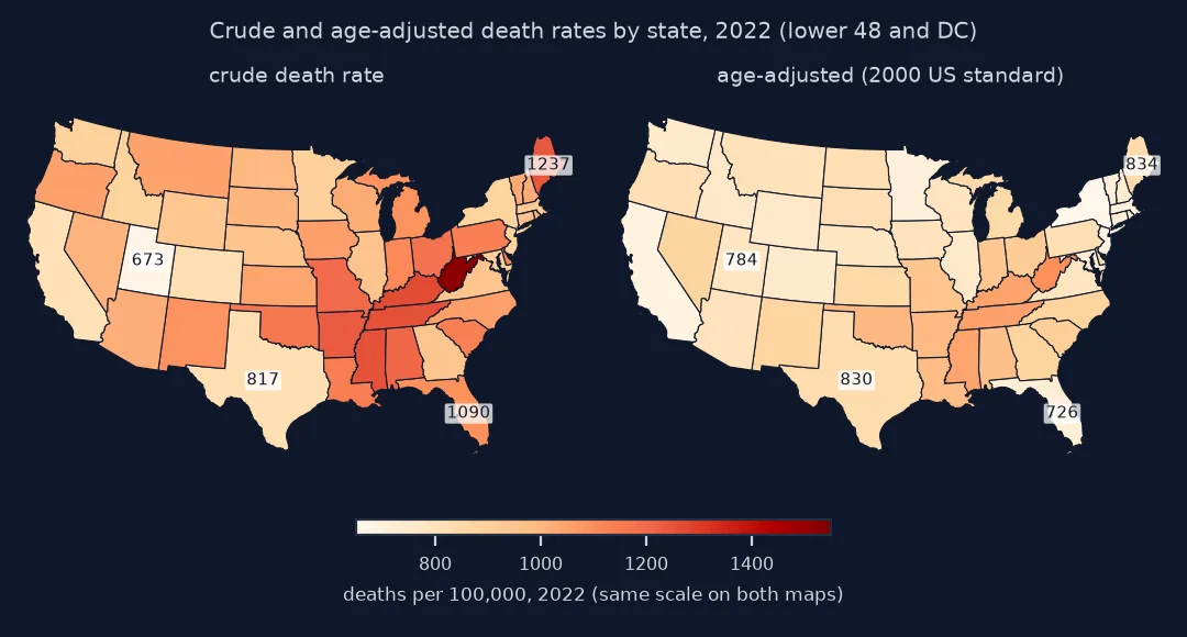
Deaths by age, standard weights, a check against published rates
1. Get deaths by age, and read the footnotes
The CDC dataset of provisional deaths by state and age (9bhg-hcku) has the 11 age groups NCHS uses for age adjustment. Two of its conventions matter: New York City is reported separately from the rest of New York State, and counts from 1 to 9 are suppressed:
print(f"New York without the city: {raw[raw.state == 'New York'].deaths.sum():,.0f} deaths; "
      f"New York City: {raw[raw.state == 'New York City'].deaths.sum():,.0f}")
print("suppressed cells:", DEATHS.isna().sum().sum(), DEATHS.columns[DEATHS.isna().any()].tolist())
for fill in (0, 9):
    a = age_adjusted(DEATHS.fillna(fill), POP, W)
    print(f"  filled with {fill}: Rhode Island {a['Rhode Island']:.1f}, Vermont {a['Vermont']:.1f}")
New York without the city: 111,993 deaths; New York City: 60,596
suppressed cells: 6 ['1-4 years', '5-14 years']
filled with 0: Rhode Island 736.0, Vermont 725.5
filled with 9: Rhode Island 738.4, Vermont 727.7
The suppressed cells are young children in small states. Filling them with the extremes, 0 or 9, moves Rhode Island's adjusted rate by 2.4 per 100,000: small, but not nothing, because the standard population gives children a large weight. Report the range, or use a fixed value such as 5 and say so.
2. Build the standard weights
The 2000 US standard population is published by NCHS and distributed by SEER in 19 age groups; merge them into the same 11 groups as the deaths:
print(f"2000 US standard million: {STD.sum():,} people in {len(STD)} groups → {len(W)} groups")
print(W.map("{:.4f}".format).to_string())
2000 US standard million: 1,000,000 people in 19 groups → 11 groups
Under 1 year 0.0138
1-4 years 0.0553
5-14 years 0.1456
15-24 years 0.1386
25-34 years 0.1356
35-44 years 0.1626
45-54 years 0.1348
55-64 years 0.0872
65-74 years 0.0660
75-84 years 0.0448
85 years and over 0.0155
3. Check the result against the published rate
NCHS published an age-adjusted death rate of 798.8 per 100,000 for the United States in 2022. Compute the national figure the same way, with both vintages of Census population estimate for 2022:
us = deaths_by_age(api, "United States")
for vintage, P in (("Vintage 2022", POP_V2022_US), ("Vintage 2023", POP_V2023_US)):
    r = (us / P * 1e5 * W).sum()
    print(f"{vintage}: adjusted rate {r:.1f}; population 85 and over {P.iloc[-1]:,}")
print(f"deaths: {us.sum():,.0f} provisional, against 3,279,857 final")
Vintage 2022: adjusted rate 801.2; population 85 and over 6,485,868
Vintage 2023: adjusted rate 816.9; population 85 and over 6,058,858
deaths: 3,288,942 provisional, against 3,279,857 final
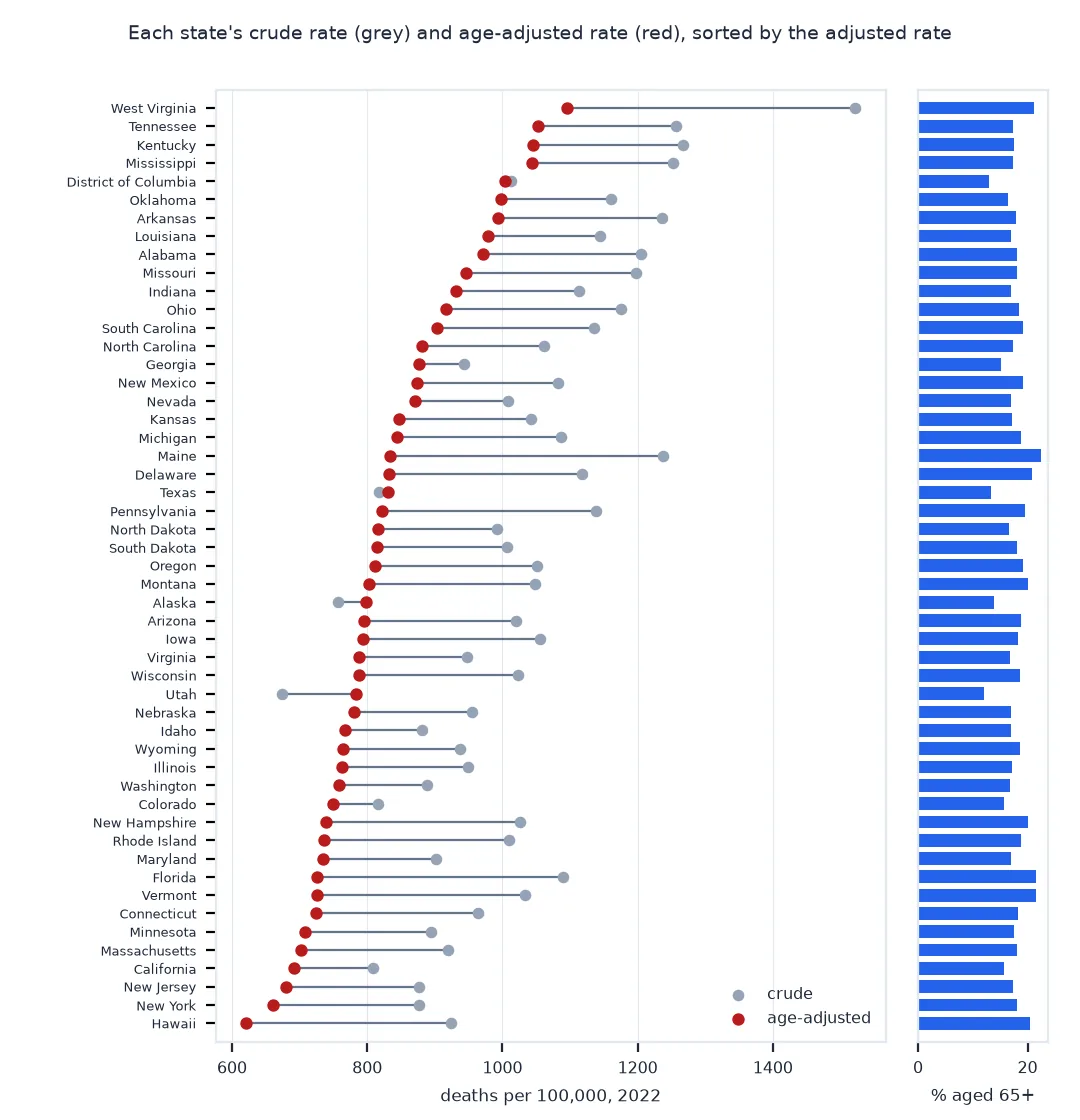
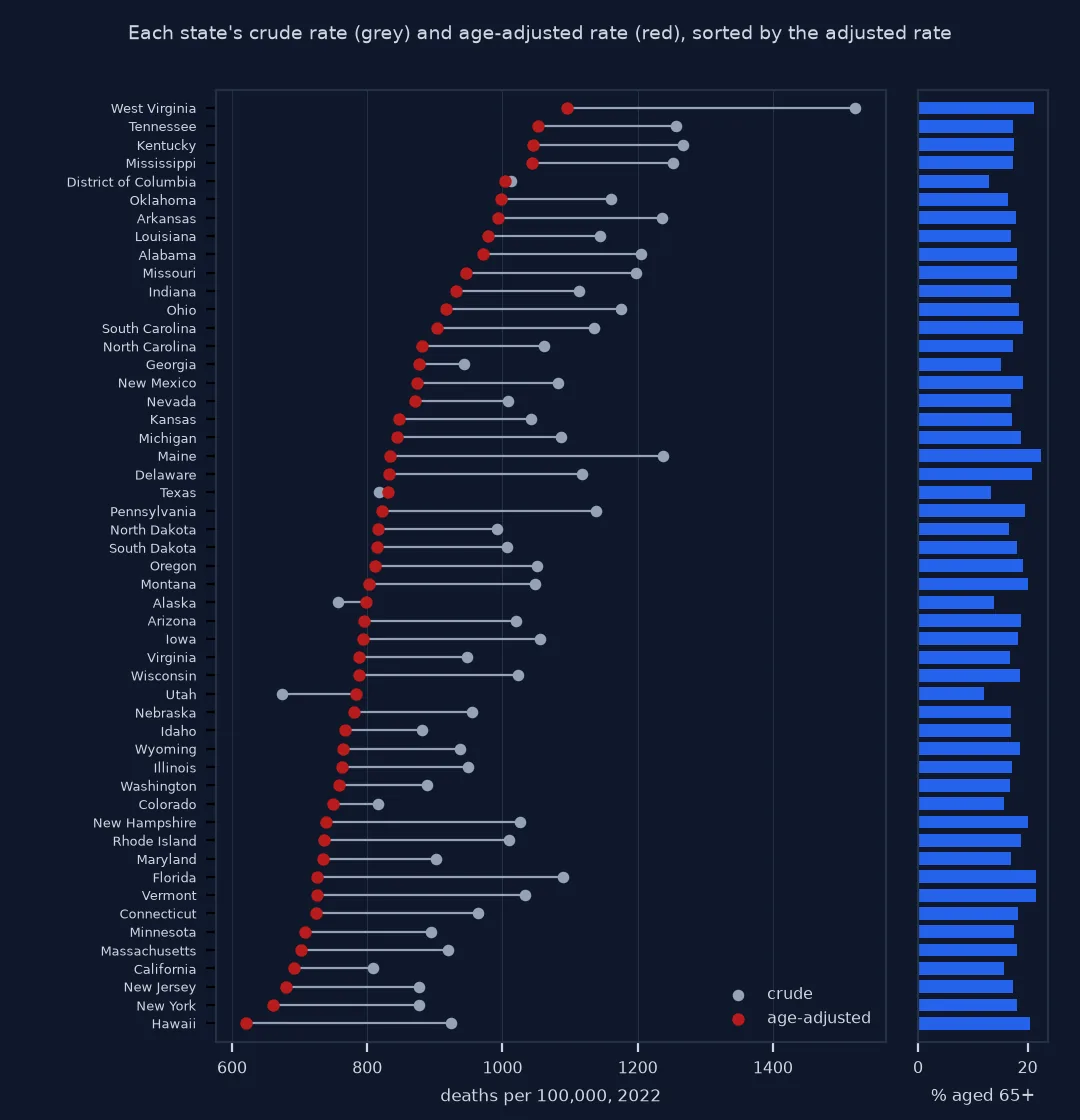
The population vintage matters. NCHS computed 2022 rates with the Vintage 2022 estimates. The following year the Census Bureau revised its estimate of people aged 85 and over in 2022 downwards by 427,010, which raises the 85+ death rate and the whole adjusted rate. With the vintage NCHS used, the remaining difference is the provisional deaths, 0.3% more than the final count.
Intervals and the states that move most
The data used on this page
Deaths by state, age group and year from the CDC dataset Provisional COVID-19 Deaths by Sex and Age (total_deaths is deaths from all causes), the Census Bureau's state population estimates by single year of age (sc-est2022-alldata6.csv, Vintage 2022, and Vintage 2023 for comparison), and the 2000 US standard population from SEER (standard 201, the 2000 US standard million).
from pathlib import Path

import numpy as np
import pandas as pd
import requests

Path("data").mkdir(exist_ok=True)
SRC = {"sc-est2022-alldata6.csv": "https://www2.census.gov/programs-surveys/popest/datasets/2020-2022/state/asrh/sc-est2022-alldata6.csv",
       "sc-est2023-alldata6.csv": "https://www2.census.gov/programs-surveys/popest/datasets/2020-2023/state/asrh/sc-est2023-alldata6.csv",
       "stdpop.19ages.txt": "https://seer.cancer.gov/stdpopulations/stdpop.19ages.txt"}
for name, url in SRC.items():
    if not Path("data", name).exists():
        Path("data", name).write_bytes(requests.get(url, timeout=300).content)

AGES = ["Under 1 year", "1-4 years", "5-14 years", "15-24 years", "25-34 years", "35-44 years",
        "45-54 years", "55-64 years", "65-74 years", "75-84 years", "85 years and over"]
EDGES = [0, 1, 5, 15, 25, 35, 45, 55, 65, 75, 85]

api = pd.DataFrame(requests.get("https://data.cdc.gov/resource/9bhg-hcku.json", params={
    "$where": "`group` = 'By Year' AND year = '2022' AND sex = 'All Sexes'",
    "$select": "state, age_group, total_deaths", "$limit": 5000}, timeout=120).json())
raw = api[api.age_group.isin(AGES)].assign(deaths=lambda d: d.total_deaths.astype(float))

def deaths_by_age(api, state):
    d = api[(api.state == state) & api.age_group.isin(AGES)]
    return d.set_index("age_group").total_deaths.astype(float)[AGES]

DEATHS = (raw.assign(state=raw.state.replace({"New York City": "New York"}))          # NYC is reported on its own
             .groupby(["state", "age_group"]).deaths.sum(min_count=1).unstack()[AGES]
             .drop(index=["United States", "Puerto Rico"]))

def pop_by_age(file):
    p = pd.read_csv(f"data/{file}")
    p = p[(p.SUMLEV == 40) & (p.SEX == 0) & (p.ORIGIN == 0)]                  # the 50 states and DC
    p = p.groupby(["NAME", "AGE"]).POPESTIMATE2022.sum().unstack()
    groups = np.searchsorted(EDGES, p.columns, side="right") - 1          # single years of age → 11 groups
    return p.T.groupby(groups).sum().T.set_axis(AGES, axis=1)

POP = pop_by_age("sc-est2022-alldata6.csv").loc[DEATHS.index]
POP_V2022_US = POP.sum()
POP_V2023_US = pop_by_age("sc-est2023-alldata6.csv").sum()

std = pd.read_fwf("data/stdpop.19ages.txt", widths=[3, 3, 8], names=["standard", "age", "pop"], dtype={"standard": str})
STD = std[std.standard == "201"]["pop"].to_numpy()                       # 0, 1–4, 5–9, ..., 85+
W = pd.Series(np.add.reduceat(STD, [0, 1, 2, 4, 6, 8, 10, 12, 14, 16, 18]) / STD.sum(), index=AGES)
print(f"{len(DEATHS)} areas (the 50 states and DC); {DEATHS.sum().sum():,.0f} deaths; population {POP.sum().sum():,}")
51 areas (the 50 states and DC); 3,288,902 deaths; population 333,287,557
Example 1: confidence intervals
Death counts are treated as Poisson, so the variance of an adjusted rate is the weighted sum of each age group's variance:
se = np.sqrt(((W ** 2) * DEATHS.fillna(0) / POP ** 2).sum(axis=1)) * 1e5
R["ci95"] = 1.96 * se
print(R.sort_values("ci95", ascending=False).head(4)[["adjusted", "ci95"]].round(1).to_string())
print(f"median half-width {R.ci95.median():.1f} per 100,000")
adjusted ci95
state
District of Columbia 1003.1 24.1
Alaska 798.5 21.9
Wyoming 763.7 20.8
North Dakota 815.7 18.7
median half-width 7.9 per 100,000
At state level the intervals are narrow, a median of 7.9 per 100,000 either side and 24 for DC, the smallest population, so most of the ranking of states is real. For counties and tracts they widen quickly, and NCHS switches from this normal approximation to gamma intervals when the deaths number fewer than 100.
Example 2: the states that move most
R["moved"] = R.rank_crude - R.rank_adjusted
print(R.reindex(R.moved.abs().sort_values(ascending=False).index).head(8)[["crude", "adjusted", "rank_crude", "rank_adjusted"]].to_string())
crude adjusted rank_crude rank_adjusted
state
Florida 1090.3 726.5 16 43
Texas 817.3 830.1 47 22
District of Columbia 1012.5 1003.1 28 5
Georgia 942.7 876.4 37 15
Alaska 756.6 798.5 50 28
Vermont 1032.7 725.5 24 44
Utah 673.4 783.7 51 33
Maine 1237.4 833.5 5 20
Crude and adjusted rates are both weighted averages
The crude rate is a weighted average of the age-specific rates, weighted by each area's own age structure. The adjusted rate is the same average with one set of weights for every area. Areas with old populations, such as Florida, Maine and Vermont, have high crude rates partly because so much of their weight sits in the oldest groups, where death rates are measured in thousands per 100,000. Young states such as Utah, Alaska and Texas have low crude rates for the opposite reason. Adjusting puts them all on the same age structure, so what remains is the difference in death rates at each age.
The adjusted rate is a comparison figure, not a count anyone experienced. Its level depends on the standard: the 2000 US standard population, used by NCHS and most US agencies, gives different numbers from the World Health Organization or European standards, and rates adjusted to different standards must not be compared. The age groups must match too: the deaths, the population and the standard all need the same 11 groups.
Population vintages, unknown ages and small numbers
- Population vintage: use the vintage of population estimates the published rates used, or recompute both; the Census Bureau revises estimates every year.
- Provisional deaths: provisional counts include some records later corrected; final NCHS data differ slightly.
- Unknown age: deaths with an unknown age are excluded from age-specific counts; here the 11 groups sum exactly to the all-ages total.
- Small numbers: below about 20 deaths, rates are unstable; NCHS flags them as unreliable.
- Puerto Rico: in the deaths data but not in the state population file used here; it needs the Puerto Rico municipio estimates.
Internal links
- Why does my death rate map show where old people live? — the symptom this fixes
- Age standardisation explained — direct and indirect standardisation and the choice of standard
FAQ
How do I calculate an age-adjusted rate in Python?
Divide deaths by population in each age group, multiply each rate by the standard population's share in that age group, and sum across age groups.
Which standard population should I use for US data?
The 2000 US standard population, which NCHS uses for all published age-adjusted rates; use the same one to compare with published figures.
Why does my age-adjusted rate not match the CDC's published figure?
Check the population estimates (vintage), the standard and its age groups, and whether the deaths are provisional or final.
Where can I get deaths by age and state?
From the CDC data portal, for example the provisional deaths by sex and age dataset, or from CDC WONDER for final data with more detail.