How to Map County Drug Overdose Death Rates in Python

On this page

Problem statement

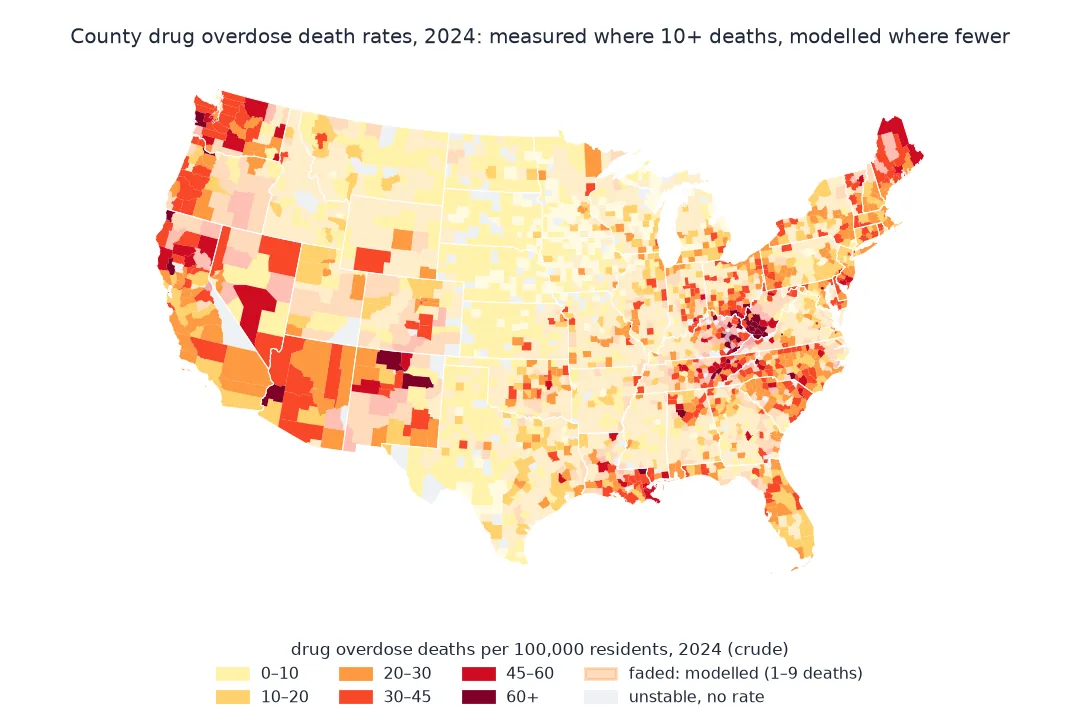
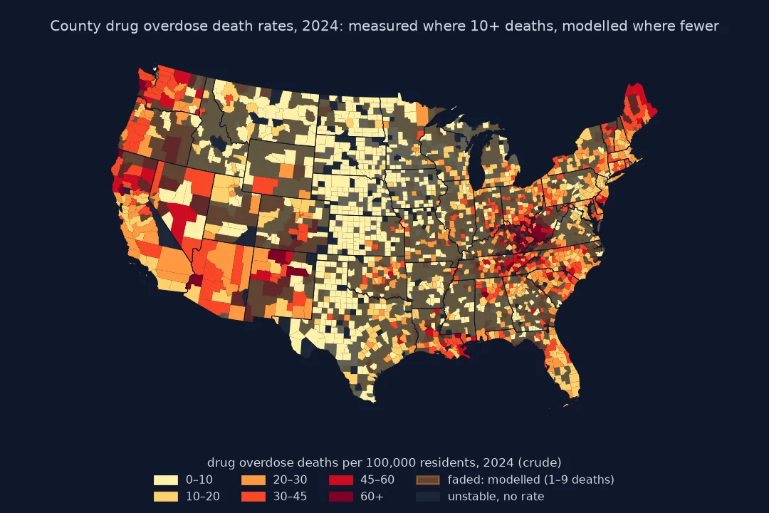
County maps of drug overdose deaths are among the most requested health maps, and the data come with three complications. Half of all counties have between one and nine deaths in a year, a range NCHS suppresses to protect confidentiality, so their counts are not published at all. The CDC fills those counties with modelled rates that borrow strength from neighbouring areas, which look exactly like measured rates in the file. And the published rates are crude, deaths per 100,000 people, not age-adjusted.

This page maps 2024 county overdose death rates from the CDC's Mapping Injury, Overdose, and Violence data, separates measured from modelled rates, and shows how uncertain the modelled ones are.

Quick answer

Parse the suppressed counts, keep the modelled flag, and join to county boundaries of the same vintage as the data:

od = soql("intent = 'Drug_OD' AND period = '2024'")
od["deaths"] = pd.to_numeric(od.count_sup, errors="coerce")       # '1-9' and '10-50' become NaN
od["rate"] = od.rate.astype(float).where(lambda r: r != -999)    # -999 marks an unstable rate
od["modelled"] = od.rate_m.astype(float) == 1
gdf = COUNTIES.merge(od[["geoid", "deaths", "count_sup", "rate", "modelled", "rate_m_ci"]], left_on="GEOID", right_on="geoid")
print(f"{len(gdf)} counties joined; measured rates (10+ deaths): {(gdf.deaths >= 10).sum()}, "
      f"no deaths: {(gdf.count_sup == '0').sum()}, modelled: {(gdf.modelled & gdf.rate.notna()).sum()}, unstable: {gdf.rate.isna().sum()}")
print(f"counties with 1-9 deaths: {(gdf.count_sup == '1-9').sum()}; with none: {(gdf.count_sup == '0').sum()}")

3141 counties joined; measured rates (10+ deaths): 1044, no deaths: 546, modelled: 1422, unstable: 129
counties with 1-9 deaths: 1547; with none: 546

Map of 2024 drug overdose death rates per 100,000 residents for counties of the lower 48 states in six classes from 0 to over 60, with modelled rates faded: the highest measured rates are in central Appalachia around West Virginia and eastern Kentucky, in parts of the Southwest, northern California, the Pacific Northwest and Maine; much of the Great Plains has no deaths or faded modelled rates; a few counties are unstable with no rate. — Measured and modelled rates on one map, the modelled ones faded.

Counts as text, measured against modelled, the kind of rate

1. Read the count column as text first

The count column mixes numbers with ranges. Converting it straight to integers fails; coercing turns the ranges into missing values, which is right as long as you then treat them as missing, not zero:

print(od.count_sup.where(od.deaths.isna()).value_counts().to_string())
n19, n1050 = (od.count_sup == "1-9").sum(), (od.count_sup == "10-50").sum()
print(f"deaths in counties with a published count: {od.deaths.sum():,.0f}; "
      f"the suppressed counties add between {n19 + 10 * n1050:,} and {9 * n19 + 50 * n1050:,} more")

count_sup
1-9      1547
10-50       4
deaths in counties with a published count: 69,140; the suppressed counties add between 1,587 and 14,123 more

2. Separate measured and modelled rates

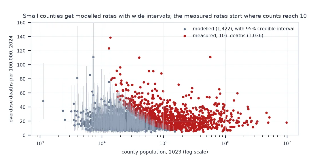
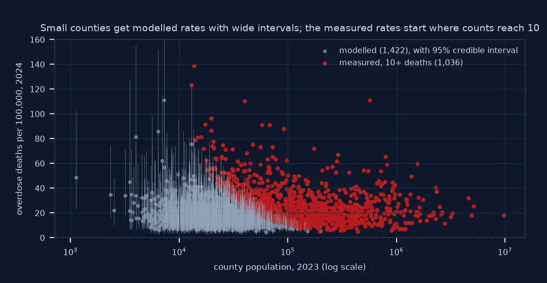
Where a county has 1 to 9 deaths, the CDC publishes a rate from a Bayesian model, with a 95% credible interval; so it does for the four counties whose count is given only as 10-50. Those intervals are wide:

m = gdf[gdf.modelled & gdf.rate.notna()].copy()
lohi = m.rate_m_ci.str.split("-", expand=True).astype(float)
m["width"] = lohi[1] - lohi[0]
print(f"modelled rates: median {m.rate.median():.1f} per 100,000, credible interval median width {m.width.median():.1f}")
measured = gdf[~gdf.modelled & gdf.rate.notna() & (gdf.deaths > 0)]
print(f"measured rates (10+ deaths): median {measured.rate.median():.1f}; range {measured.rate.min():.1f}–{measured.rate.max():.1f}")

modelled rates: median 15.3 per 100,000, credible interval median width 20.7
measured rates (10+ deaths): median 24.1; range 5.0–139.1

Scatter of county overdose death rates in 2024 against population on a log scale: modelled rates for small counties, 1,422 grey points each with a tall 95 percent credible interval, cluster between 5 and 40; measured rates, red, start around 10,000 people and spread from 5 to 139 per 100,000, narrowing as population grows. — Modelled rates are shrunk and uncertain; measured ones are noisy where counts are small.

3. Check what kind of rate it is

The data dictionary says "deaths per 100,000 people". Dividing the published counts by the rates gives the population each rate used, which can be compared with the Census estimates:

x = gdf[gdf.deaths >= 10].merge(POPEST, on="GEOID")
implied = x.deaths / x.rate * 1e5
for year in (2023, 2024):
    print(f"implied population ÷ Census {year} estimate: median {(implied / x[f'POPESTIMATE{year}']).median():.4f}")

implied population ÷ Census 2023 estimate: median 0.9977
implied population ÷ Census 2024 estimate: median 0.9907

The rates are crude. Even the 2024 rates were computed on populations within a fraction of a percent of the Census estimate for 2023. Counties with older populations will look worse than their age-specific rates justify, although overdose deaths are concentrated at working ages, so the effect is smaller than for all-cause mortality.

2023 against 2024, and the highest measured rates

The data used on this page

The CDC's Mapping Injury, Overdose, and Violence county dataset (psx4-wq38), drug overdose deaths of unintentional or undetermined intent by county of residence for 2023 and 2024, the 2021 Census cartographic boundary file of counties, which still has Connecticut's eight historical counties that the CDC data use, and the Census Bureau's county population estimates (Vintage 2024).

from pathlib import Path

import geopandas as gpd
import numpy as np
import pandas as pd
import requests

Path("data").mkdir(exist_ok=True)
SRC = {"cb_2021_us_county_5m.zip": "https://www2.census.gov/geo/tiger/GENZ2021/shp/cb_2021_us_county_5m.zip",
       "co-est2024-alldata.csv": "https://www2.census.gov/programs-surveys/popest/datasets/2020-2024/counties/totals/co-est2024-alldata.csv"}
for name, url in SRC.items():
    if not Path("data", name).exists():
        Path("data", name).write_bytes(requests.get(url, timeout=300).content)

def soql(where, page=5000):
    rows, offset = [], 0
    while True:
        part = requests.get("https://data.cdc.gov/resource/psx4-wq38.json", timeout=120,
                            params={"$where": where, "$limit": page, "$offset": offset, "$order": ":id"}).json()
        rows += part; offset += len(part)
        if len(part) < page:
            return pd.DataFrame(rows)

COUNTIES = gpd.read_file("data/cb_2021_us_county_5m.zip")
c = pd.read_csv("data/co-est2024-alldata.csv", encoding="latin-1", dtype={"STATE": str, "COUNTY": str})
POPEST = c[c.SUMLEV == 50].assign(GEOID=lambda d: d.STATE + d.COUNTY)[["GEOID", "POPESTIMATE2023", "POPESTIMATE2024"]]
print(f"{len(COUNTIES)} county boundaries (2021); {len(POPEST)} counties in the 2024 estimates")

3234 county boundaries (2021); 3144 counties in the 2024 estimates

Example 1: 2023 against 2024

prev = soql("intent = 'Drug_OD' AND period = '2023'").assign(d23=lambda d: pd.to_numeric(d.count_sup, errors="coerce"))
both = od.merge(prev[["geoid", "d23"]], on="geoid").dropna(subset=["deaths", "d23"])
both = both[(both.deaths >= 10) & (both.d23 >= 10)]
print(f"{len(both)} counties with 10+ deaths in both years: {both.deaths.sum():,.0f} deaths in 2024 against {both.d23.sum():,.0f} in 2023 "
      f"({both.deaths.sum() / both.d23.sum() - 1:+.0%}); fewer deaths in {(both.deaths < both.d23).sum()} of them")

984 counties with 10+ deaths in both years: 68,410 deaths in 2024 against 91,334 in 2023 (-25%); fewer deaths in 827 of them

Example 2: the highest measured rates

top = gdf[~gdf.modelled & (gdf.deaths >= 20)].nlargest(6, "rate")
print(top[["NAMELSAD", "STUSPS", "deaths", "rate"]].to_string(index=False))                # NAME alone has two Baltimores

         NAMELSAD STUSPS  deaths  rate
   Baltimore city     MD   628.0 111.1
Rio Arriba County     NM    44.0 110.3
      Lake County     CA    62.0  91.3
    Mercer County     WV    53.0  91.3
    Cabell County     WV    81.0  88.0
      Boyd County     KY    36.0  75.3

A county overdose map is a map of small numbers

More counties carry a modelled rate than a measured one.

A county overdose map is a map of small numbers. Most US counties are rural, and in 2024 two thirds of them, 2,093 of 3,141, recorded fewer than ten overdose deaths. A raw rate from three deaths in a county of 15,000 is 20 per 100,000, but one more death would make it 27, so the map would be dominated by noise in exactly the counties that cover most of the land. The CDC's modelled rates address this by shrinking each small county's rate towards a value informed by its neighbours, and the credible interval says how much is left uncertain. The model also protects privacy, because the published rate cannot be multiplied back into a count.

The modelled rates are estimates, not measurements, and the map should say so. A different symbol or a lighter treatment for modelled counties, or a companion map of interval widths, keeps a reader from comparing a modelled rural county with a measured city as if they were the same kind of number.

County vintage, residence and intent

County overdose map traps.

County vintage: the data use Connecticut's eight historical counties, which current boundary files do not have (see why Connecticut counties go missing); in Alaska the yearly rows have no figures for the former Valdez-Cordova area at all.
Residence: counts are by county of residence, not where the death occurred.
Intent: Drug_OD covers unintentional and undetermined-intent drug overdoses; suicides by overdose are in All_Suicide.
Provisional: recent periods are revised as records arrive; the trailing twelve months (TTM) are least complete.
Crude rates: compare counties of very different age structure with care; age-adjusted county rates need deaths by age.

Internal links

How to smooth rates with empirical Bayes — the same idea, done yourself
Why does my rate map highlight the smallest areas? — small-number noise

FAQ

Where can I get county-level drug overdose death data?

From the CDC's Mapping Injury, Overdose, and Violence dataset on data.cdc.gov, which has counts and rates by county and year, and from VSRR provisional county counts.

Why are some county overdose counts shown as 1-9?

NCHS suppresses counts from 1 to 9 to protect confidentiality; the CDC publishes a modelled rate for those counties instead.

Are CDC county overdose rates age-adjusted?

No; they are crude rates per 100,000 residents. The implied populations match the Census estimates.

How should I show modelled rates on a map?

Mark them differently from measured rates, and show their credible intervals or a companion map of uncertainty.